Functions
Forward substitution
1 2 3 4 5 6 7 8 9 10 11 12 13function x = forwardsub(L,b) % FORWARDSUB Solve a lower triangular linear system. % Input: % L lower triangular square matrix (n by n) % b right-hand side vector (n by 1) % Output: % x solution of Lx=b (n by 1 vector) n = length(L); x = zeros(n,1); for i = 1:n x(i) = ( b(i) - L(i,1:i-1) * x(1:i-1) ) / L(i,i); end
About the code
Line 12 implements (2.3.7). It contains an inner product between row of and the solution vector , using only the entries of that have already been computed.
Backward substitution
1 2 3 4 5 6 7 8 9 10 11 12 13function x = backsub(U,b) % BACKSUB Solve an upper triangular linear system. % Input: % U upper triangular square matrix (n by n) % b right-hand side vector (n by 1) % Output: % x solution of Ux=b (n by 1 vector) n = length(U); x = zeros(n,1); for i = n:-1:1 x(i) = ( b(i) - U(i,i+1:n)*x(i+1:n) ) / U(i,i); end
LU factorization (not stable)
1 2 3 4 5 6 7 8 9 10 11 12 13 14 15 16 17 18 19 20function [L, U] = lufact(A) % LUFACT LU factorization (demo only--not stable!). % Input: % A square matrix % Output: % L,U unit lower triangular and upper triangular such that LU=A n = size(A, 1); % detect the dimensions from the input L = eye(n); % ones on main diagonal, zeros elsewhere U = zeros(n, n); A_k = A; % make a working copy % Reduction by outer products for k = 1:n-1 U(k, :) = A_k(k, :); L(:, k) = A_k(:,k) / U(k, k); A_k = A_k - L(:, k) * U(k, :); end U(n, n) = A_k(n, n); L = tril(L); U = triu(U); % force exact triangularity
LU factorization with partial pivoting
1 2 3 4 5 6 7 8 9 10 11 12 13 14 15 16 17 18 19 20 21 22 23 24 25function [L, U, p] = plufact(A) % PLUFACT Pivoted LU factorization % Input: % A square matrix % Output: % L unit lower triangular % U upper triangular % p row permutation vector such that A(p,:) = L*U n = size(A, 1); L = zeros(n, n); U = zeros(n, n); p = zeros(1, n); A_k = A; % Reduction by outer products for k = 1:n [~, p(k)] = max(abs(A_k(:, k))); U(k, :) = A_k(p(k), :); L(:, k) = A_k(:, k) / U(k, k); if k < n A_k = A_k - L(:, k) * U(k, :); end end L = tril(L(p, :)); U = triu(U);
Examples
2.1 Polynomial interpolation
Example 2.1.1
We create two column vectors for data about the population of China. The first has the years of census data and the other has the population, in millions of people.
year = [1982; 2000; 2010; 2015];
pop = [1008.18; 1262.64; 1337.82; 1374.62];
It’s convenient to measure time in years since 1980.
t = year - 1980;
y = pop;
Now we have four data points , so and we seek an interpolating cubic polynomial. We construct the associated Vandermonde matrix:
V = vander(t)To solve for the vector of polynomial coefficients, we use a backslash to solve the linear system:
Tip
A backslash \ is used to solve a linear system of equations.
c = V \ yThe algorithms used by the backslash operator are the main topic of this chapter. As a check on the solution, we can compute the residual.
y - V * cUsing floating-point arithmetic, it is not realistic to expect exact equality of quantities; a relative difference comparable to is all we can look for.
By our definitions, the elements of c are coefficients in descending-degree order for the interpolating polynomial. We can use the polynomial to estimate the population of China in 2005:
p = @(t) polyval(c, t - 1980);  % include the 1980 time shift
p(2005)The official population value for 2005 was 1303.72, so our result is rather good.
We can visualize the interpolation process. First, we plot the data as points.
Tip
The scatter function creates a scatter plot of points; you can specify a line connecting the points as well.
scatter(year, y)
xlabel("years since 1980")
ylabel("population (millions)")
title("Population of China")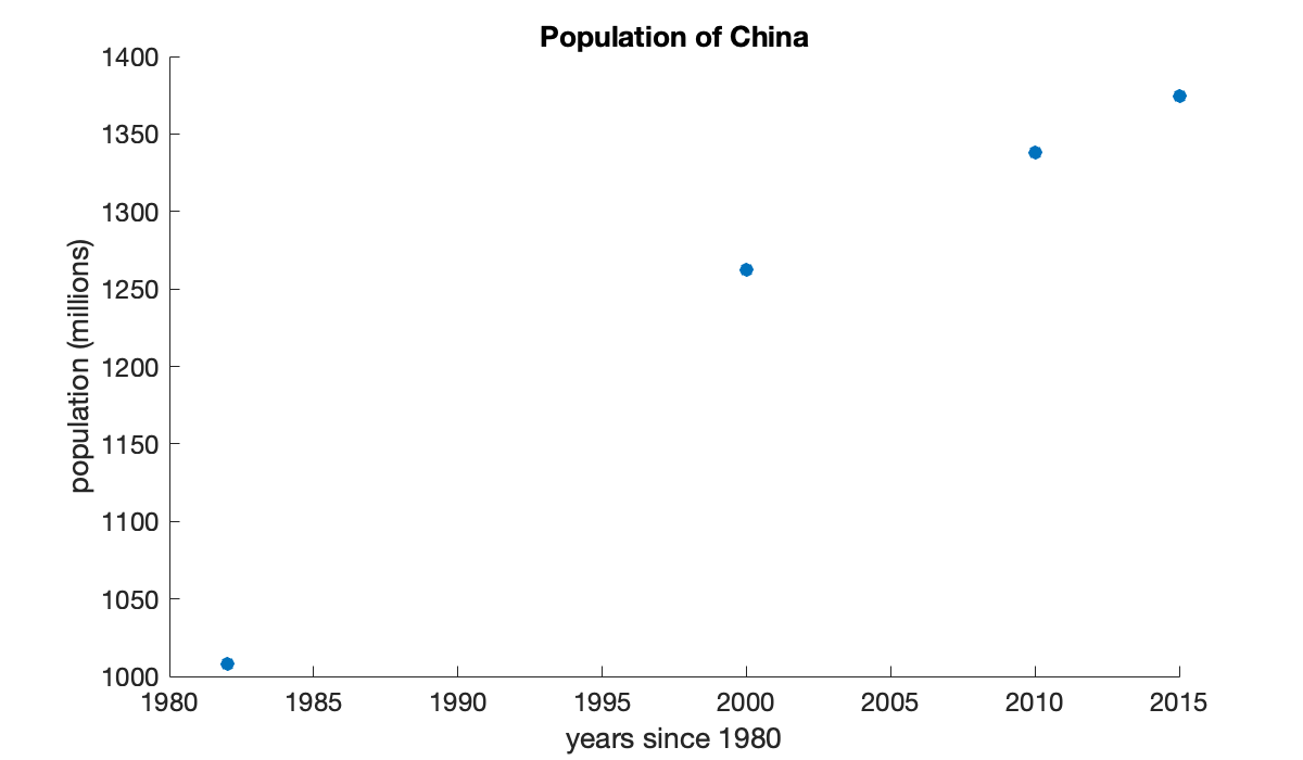
We want to superimpose a plot of the polynomial. We do that by evaluating it at a vector of points in the interval.
Tip
The linspace function constructs evenly spaced values given the endpoints and the number of values.
tt = linspace(1980, 2015, 500);    % 500 times in the interval [1980, 2015]
yy = p(tt);                        % evaluate p at all the vector elements
yy(1:4)Now we use plot! to add to the current plot, rather than replacing it.
Tip
Use hold on to add to an existing plot rather than replacing it.
The plot function plots lines connecting the given and values; you can also specify markers at the points.
hold on
plot(tt, yy)
legend("data", "interpolant", "location", "northwest");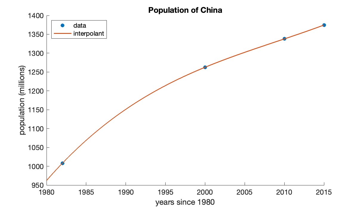
2.2 Computing with matrices
Example 2.2.1
In MATLAB, every numerical value is treated like a matrix. A matrix with one row or one column is interpreted as a vector, and a matrix is interpreted as a scalar.
Square brackets are used to enclose elements of a matrix or vector. Use spaces for horizontal concatenation, and semicolons or new lines to indicate vertical concatenation.
Tip
The size function returns the number of rows and columns in a matrix. Use length to get the number of elements in a vector or matrix.
A = [
    1       2      3             4      5;
    50     40     30            20     10
    pi sqrt(2) exp(1) (1+sqrt(5))/2 log(3)
]m, n = size(A)Unrecognized function or variable 'm'.x = [ 3, 3, 0, 1, 0 ]; % row vector
size(x)Concatenated elements within brackets may be matrices or vectors for a block representation, as long as all the block sizes are compatible.
[ x x ][ x; x ]The zeros and ones functions construct matrices with entries all zero or one, respectively.
B = [ zeros(3, 2) ones(3, 1) ]A single quote ' after a matrix returns its adjoint. For real matrices, this is the transpose; for complex-valued matrices, the elements are also conjugated.
A'There are many convenient shorthand ways of building vectors and matrices other than entering all of their entries directly or in a loop. To get a range with evenly spaced entries between two endpoints, you have two options. One is to use a colon :.
y = 1:4 % start:stopz = 0:3:12 % start:step:stopInstead of specifying the step size, you can give the number of points in the range if you use linspace.
s = linspace(-1, 1, 5) % row resultAccessing an element is done by giving one (for a vector) or two (for a matrix) index values within parentheses.
Tip
The end keyword refers to the last element in a dimension. It saves you from having to compute and store the size of the matrix first.
a = A(2, end-1)x(2)The indices can be vectors or ranges, in which case a block of the matrix is accessed.
A(1:2, end-2:end) % first two rows, last three columnsIf a dimension has only the index : (a colon), then it refers to all the entries in that dimension of the matrix.
A(:, 1:2:end) % all of the odd columnsThe matrix and vector senses of addition, subtraction, scalar multiplication, multiplication, and power are all handled by the usual symbols.
Tip
Use diag to construct a matrix by its diagonals. A more general syntax puts elements on super- or subdiagonals.
B = diag([-1, 0, -5]) % create a diagonal matrixsize(A)
size(B)BA = B * A % matrix productA * B causes an error here, because the dimensions aren’t compatible.
Tip
Errors are formally called exceptions in Julia.
A * B % throws an errorError using *
Incorrect dimensions for matrix multiplication. Check that the number of columns in the first matrix matches the number of rows in the second matrix. To operate on each element of the matrix individually, use TIMES (.*) for elementwise multiplication.A square matrix raised to an integer power is the same as repeated matrix multiplication.
B^3 % same as B*B*BSometimes one instead wants to treat a matrix or vector as a mere array and simply apply a single operation to each element of it. For multiplication, division, and power, the corresponding operators start with a dot.
C = -A;Because both matrices are , A * C would be an error here, but elementwise operations are fine.
elementwise = A .* CThe two operands of a dot operator have to have the same size—unless one is a scalar, in which case it is expanded or broadcast to be the same size as the other operand.
x_to_two = x .^ 2two_to_x = 2 .^ xTip
Most of the mathematical functions, such as cos, sin, log, exp, and sqrt, can operate elementwise on vectors and matrices.
cos(pi * x)2.3 Linear systems
Example 2.3.2
For a square matrix , the syntax A \ b is mathematically equivalent to .
A = [1 0 -1; 2 2 1; -1 -3 0]b = [1; 2; 3]x = A \ bOne way to check the answer is to compute a quantity known as the residual. It is (ideally) close to machine precision (relative to the elements in the data).
residual = b - A*xIf the matrix is singular, you may get a warning and nonsense result.
A = [0 1; 0 0]
b = [1; -1]
x = A \ bIn this case, we can check that the rank of is less than its number of columns, indicating singularity.
Tip
The function rank computes the rank of a matrix. However, it is numerically unstable for matrices that are nearly singular, in a sense to be defined in a later section.
rank(A)A linear system with a singular matrix might have no solution or infinitely many solutions, but in either case, backslash will fail. Moreover, detecting singularity is a lot like checking whether two floating-point numbers are exactly equal: because of roundoff, it could be missed. In Conditioning of linear systems we’ll find a robust way to fully describe this situation.
Example 2.3.3
It’s easy to get just the lower triangular part of any matrix using the tril function.
Tip
Use tril to return a matrix that zeros out everything above the main diagonal. The triu function zeros out below the diagonal.
A = randi(9, 5, 5);
L = tril(A)We’ll set up and solve a linear system with this matrix.
b = ones(5);
x = forwardsub(L, b)It’s not clear how accurate this answer is. However, the residual should be zero or comparable to .
b - L * xNext, we’ll engineer a problem to which we know the exact answer.
Tip
The eye function creates an identity matrix. The diag function uses 0 as the main diagonal, positive integers as superdiagonals, and negative integers as subdiagonals.
alpha = 0.3;
beta = 2.2;
U = eye(5) + diag([-1 -1 -1 -1], 1);
U(1, [4, 5]) = [alpha - beta, beta]x_exact = ones(5);
b = [alpha; 0; 0; 0; 1];Now we use backward substitution to solve for , and compare to the exact solution we know already.
x = backsub(U, b);
err = x - x_exactEverything seems OK here. But another example, with a different value for β, is more troubling.
alpha = 0.3;
beta = 1e12;
U = eye(5) + diag([-1 -1 -1 -1], 1);
U(1, [4, 5]) = [alpha - beta, beta];
b = [alpha; 0; 0; 0; 1];

x = backsub(U, b);
err = x - x_exactIt’s not so good to get 4 digits of accuracy after starting with sixteen! The source of the error is not hard to track down. Solving for performs in the first row. Since is so much smaller than , this a recipe for losing digits to subtractive cancellation.
2.4 LU factorization
Example 2.4.2
We explore the outer product formula for two random triangular matrices.
L = tril( randi(9, 3, 3) )U = triu( randi(9, 3, 3) )Here are the three outer products in the sum in (2.4.4):
L(:, 1) * U(1, :)L(:, 2) * U(2, :)L(:, 3) * U(3, :)Simply because of the triangular zero structures, only the first outer product contributes to the first row and first column of the entire product.
Example 2.4.3
For illustration, we work on a matrix. We name it with a subscript in preparation for what comes.
A_1 = [
     2    0    4     3
    -4    5   -7   -10
     1   15    2   -4.5
    -2    0    2   -13
    ];
L = eye(4);
U = zeros(4, 4);
Now we appeal to (2.4.5). Since , we see that the first row of is just the first row of .
U(1, :) = A_1(1, :)From (2.4.6), we see that we can find the first column of from the first column of .
L(:, 1) = A_1(:, 1) / U(1, 1)We have obtained the first term in the sum (2.4.4) for , and we subtract it away from .
A_2 = A_1 - L(:, 1) * U(1, :)Now If we ignore the first row and first column of the matrices in this equation, then in what remains we are in the same situation as at the start. Specifically, only has any effect on the second row and column, so we can deduce them now.
U(2, :) = A_2(2, :)
L(:, 2) = A_2(:, 2) / U(2, 2)If we subtract off the latest outer product, we have a matrix that is zero in the first two rows and columns.
A_3 = A_2 - L(:, 2) * U(2, :)Now we can deal with the lower right submatrix of the remainder in a similar fashion.
U(3, :) = A_3(3, :);
L(:, 3) = A_3(:, 3) / U(3, 3);
A_4 = A_3 - L(:, 3) * U(3, :)Finally, we pick up the last unknown in the factors.
U(4, 4) = A_4(4, 4);We now have all of ,
Land all of ,
UWe can verify that we have a correct factorization of the original matrix by computing the backward error:
A_1 - L * UIn floating point, we cannot expect the difference to be exactly zero as we found in this toy example. Instead, we would be satisfied to see that each element of the difference above is comparable in size to machine precision.
Example 2.4.4
Here are the data for a linear system .
A = [2 0 4 3; -4 5 -7 -10; 1 15 2 -4.5; -2 0 2 -13];
b = [4; 9; 9; 4];
We apply Function 2.4.1 and then do two triangular solves.
[L, U] = lufact(A)
z = forwardsub(L, b);
x = backsub(U, z);A check on the residual assures us that we found the solution.
b - A * x2.5 Efficiency of matrix computations
Example 2.5.4
Here is a straightforward implementation of matrix-vector multiplication.
n = 6;
A = magic(n);
x = ones(n,1);
y = zeros(n,1);
for i = 1:n
    for j = 1:n
        y(i) = y(i) + A(i,j)*x(j);   % 2 flops
    end
end
Each of the loops implies a summation of flops. The total flop count for this algorithm is
Since the matrix has elements, all of which have to be involved in the product, it seems unlikely that we could get a flop count that is smaller than in general.
Let’s run an experiment with the built-in matrix-vector multiplication, using tic and toc to time the operation.
n = (500:500:5000)';
t = zeros(size(n));
for k = 1:length(n)
    A = randn(n(k), n(k));  x = randn(n(k), 1);
    tic    % start a timer
    for j = 1:200      % repeat 100 times
        A*x;
    end
    time = toc;           % read the timer
    t(k) = time / 200;   % seconds per instance
end
The reason for doing multiple repetitions at each value of in the loop above is to avoid having times so short that the resolution of the timer is significant.
table(n, t, 'variablenames', ["size", "time"])Looking at the timings just for and , they have ratio
Tip
The expression n==5000 here produces a vector of Boolean (true/false) values the same size as n. This result is used to index within t, accessing only the value for which the comparison is true.
t(n==5000) / t(n==2500)If the run time is dominated by flops, then we expect this ratio to be
Example 2.5.5
Let’s repeat the previous experiment for more, and larger, values of .
n = (400:400:6000)';
t = zeros(size(n));
for k = 1:length(n)
    A = randn(n(k), n(k));  x = randn(n(k), 1);
    tic    % start a timer
    for j = 1:100      % repeat ten times
        A*x;
    end
    time = toc;          % read the timer
    t(k) = time / 100;   % seconds per instance
end
Plotting the time as a function of on log-log scales is equivalent to plotting the logs of the variables.
clf    % clear any existing figure
loglog(n, t, 'o-')
xlabel('size of matrix')
ylabel('time (sec)')
title('Timing of matrix-vector multiplications')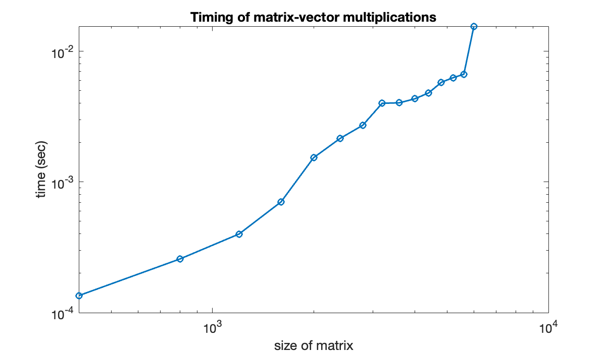
You can see that while the full story is complicated, the graph is trending to a straight line of positive slope. For comparison, we can plot a line that represents growth exactly. (All such lines have slope equal to 2.)
hold on
loglog(n, 0.5 * t(end) * (n / n(end)).^2, 'k--')
axis tight
legend('data', 'O(n^2)', 'location', 'southeast')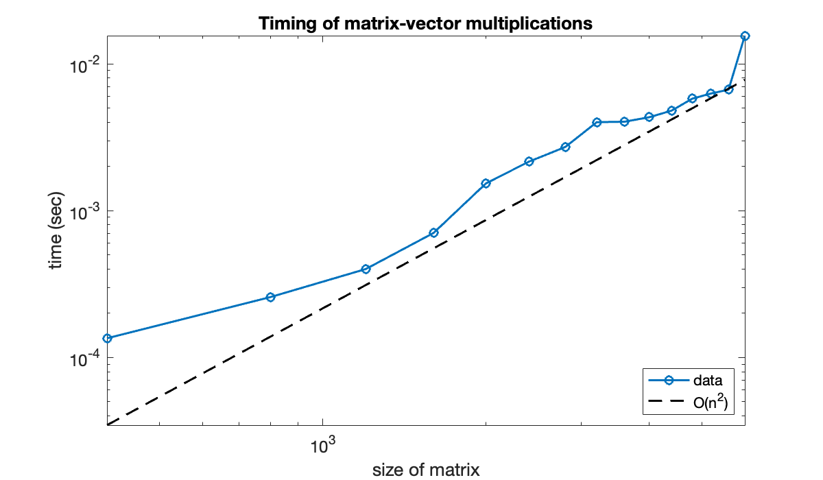
Example 2.5.6
We’ll test the conclusion of flops experimentally, using the built-in lu function instead of the purely instructive lufact.
Tip
The first time a function is invoked, there may be significant time needed to compile it in memory. Thus, when timing a function, run it at least once before beginning the timing.
n = (200:100:2400)';
t = zeros(size(n));
for k = 1:length(n)
    A = randn(n(k), n(k));
    tic    % start a timer
    for j = 1:6,  [L, U] = lu(A);  end
    time = toc;
    t(k) = time / 6;
end
We plot the timings on a log-log graph and compare it to . The result could vary significantly from machine to machine, but in theory the data should start to parallel the line as .
clf
loglog(n, t, 'o-')
hold on
loglog(n, 0.5 * t(end) * (n/n(end)).^3, 'k--')
axis tight
xlabel('size of matrix'), ylabel('time (sec)')
title('Timing of LU factorization')
legend('lu','O(n^3)','location','southeast');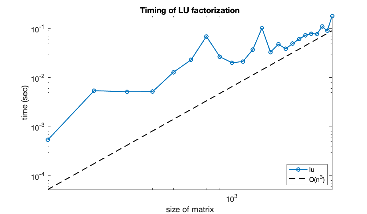
2.6 Row pivoting
Example 2.6.1
Here is a previously encountered matrix that factors well.
A = [
    2 0 4 3
    -4 5 -7 -10
    1 15 2 -4.5
    -2 0 2 -13
    ];
[L, U] = lufact(A);
LIf we swap the second and fourth rows of , the result is still nonsingular. However, the factorization now fails.
A([2, 4], :) = A([4, 2], :);    % swap rows 2 and 4
[L, U] = lufact(A);
LThe presence of NaN in the result indicates that some impossible operation was required. The source of the problem is easy to locate. We can find the first outer product in the factorization just fine:
U(1, :) = A(1, :);
L(:, 1) = A(:, 1) / U(1, 1)
A = A - L(:, 1) * U(1, :)The next step is U(2, :) = A(2, :), which is also OK. But then we are supposed to divide by U(2, 2), which is zero. The algorithm cannot continue.
Example 2.6.2
Here is the trouble-making matrix from Demo 2.6.1.
A_1 = [2 0 4 3; -2 0 2 -13; 1 15 2 -4.5; -4 5 -7 -10]We now find the largest candidate pivot in the first column. We don’t care about sign, so we take absolute values before finding the max.
Tip
The second output of max returns the location of the largest element of a vector. The ~ symbol is used to ignore the value of the first output.
[~, i] = max( abs(A_1(:, 1)) )This is the row of the matrix that we extract to put into . That guarantees that the division used to find will be valid.
L = zeros(4, 4);
U = zeros(4, 4);
U(1, :) = A_1(i, :);
L(:, 1) = A_1(:, 1) / U(1, 1);
A_2 = A_1 - L(:, 1) * U(1, :)Observe that has a new zero row and zero column, but the zero row is the fourth rather than the first. However, we forge on by using the largest possible pivot in column 2 for the next outer product.
[~, i] = max( abs(A_2(:, 2)) )
U(2, :) = A_2(i, :);
L(:, 2) = A_2(:, 2) / U(2, 2);
A_3 = A_2 - L(:, 2) * U(2, :)Now we have zeroed out the third row as well as the second column. We can finish out the procedure.
[~, i] = max( abs(A_3(:, 3)) )
U(3, :) = A_3(i, :);
L(:, 3) = A_3(:, 3) / U(3, 3);
A_4 = A_3 - L(:, 3) * U(3, :)[~, i] = max( abs(A_4(:, 4)) )
U(4, :) = A_4(i, :);
L(:, 4) = A_4(:, 4) / U(4, 4);We do have a factorization of the original matrix:
A_1 - L * UAnd has the required structure:
UHowever, the triangularity of has been broken.
LExample 2.6.3
Here again is the matrix from Demo 2.6.2.
A = [2 0 4 3; -2 0 2 -13; 1 15 2 -4.5; -4 5 -7 -10]As the factorization proceeded, the pivots were selected from rows 4, 3, 2, and finally 1. If we were to put the rows of into that order, then the algorithm would run exactly like the plain LU factorization from LU factorization.
B = A([4, 3, 2, 1], :);
[L, U] = lufact(B);
We obtain the same as before:
UAnd has the same rows as before, but arranged into triangular order:
LExample 2.6.4
The third output of plufact is the permutation vector we need to apply to .
A = randi(20, 4, 4);
[L, U, p] = plufact(A);
A(p, :) - L * U % should be ≈ 0Given a vector , we solve by first permuting the entries of and then proceeding as before.
b = rand(4, 1);
z = forwardsub(L, b(p));
x = backsub(U, z)A residual check is successful:
b - A*xExample 2.6.5
With the syntax A \ b, the matrix A is PLU-factored, followed by two triangular solves.
A = randn(500, 500);    % 500x500 with normal random entries
tic; for k=1:50; A \ rand(500, 1); end; toc
Elapsed time is 0.591412 seconds.
In Efficiency of matrix computations we showed that the factorization is by far the most costly part of the solution process. A factorization object allows us to do that costly step only once per unique matrix.
[L, U, p] = lu(A, 'vector');    % keep factorization result
tic
for k=1:50
    b = rand(500, 1);
    U \ (L \ b(p));
end
toc
Elapsed time is 0.010308 seconds.
Example 2.6.6
We construct a linear system for this matrix with and exact solution :
ep = 1e-12
A = [-ep 1; 1 -1];
b = A * [1; 1];We can factor the matrix without pivoting and solve for .
[L, U] = lufact(A);
x = backsub( U, forwardsub(L, b) )Note that we have obtained only about 5 accurate digits for . We could make the result even more inaccurate by making ε even smaller:
ep = 1e-20; A = [-ep 1; 1 -1];
b = A * [1; 1];
[L, U] = lufact(A);
x = backsub( U, forwardsub(L, b) )This effect is not due to ill conditioning of the problem—a solution with PLU factorization works perfectly:
A \ b2.7 Vector and matrix norms
Example 2.7.1
x = [2; -3; 1; -1];
twonorm = norm(x) % or norm(x, 2)infnorm = norm(x, Inf)onenorm = norm(x, 1)Example 2.7.2
A = [ 2 0; 1 -1 ]The default matrix norm is the 2-norm.
twonorm = norm(A)You can get the 1-norm as well.
onenorm = norm(A, 1)According to (2.7.15), the matrix 1-norm is equivalent to the maximum of the sums down the columns (in absolute value).
Tip
Use sum to sum along a dimension of a matrix. The max and min functions also work along one dimension.
% Sum down the rows (1st matrix dimension):
max( sum(abs(A), 1) )Similarly, we can get the ∞-norm and check our formula for it.
infnorm = norm(A, Inf)% Sum across columns (2nd matrix dimension):
max( sum(abs(A), 2) )Next we illustrate a geometric interpretation of the 2-norm. First, we will sample a lot of vectors on the unit circle in .
Tip
You can use functions as values, e.g., as elements of a vector.
theta = linspace(0, 2*pi, 601);
x = [ cos(theta); sin(theta) ];    % 601 unit column vectors
clf
subplot(1, 2, 1)
plot(x(1, :), x(2, :)), axis equal
title('Unit circle in 2-norm')
xlabel('x_1')
ylabel(('x_2'));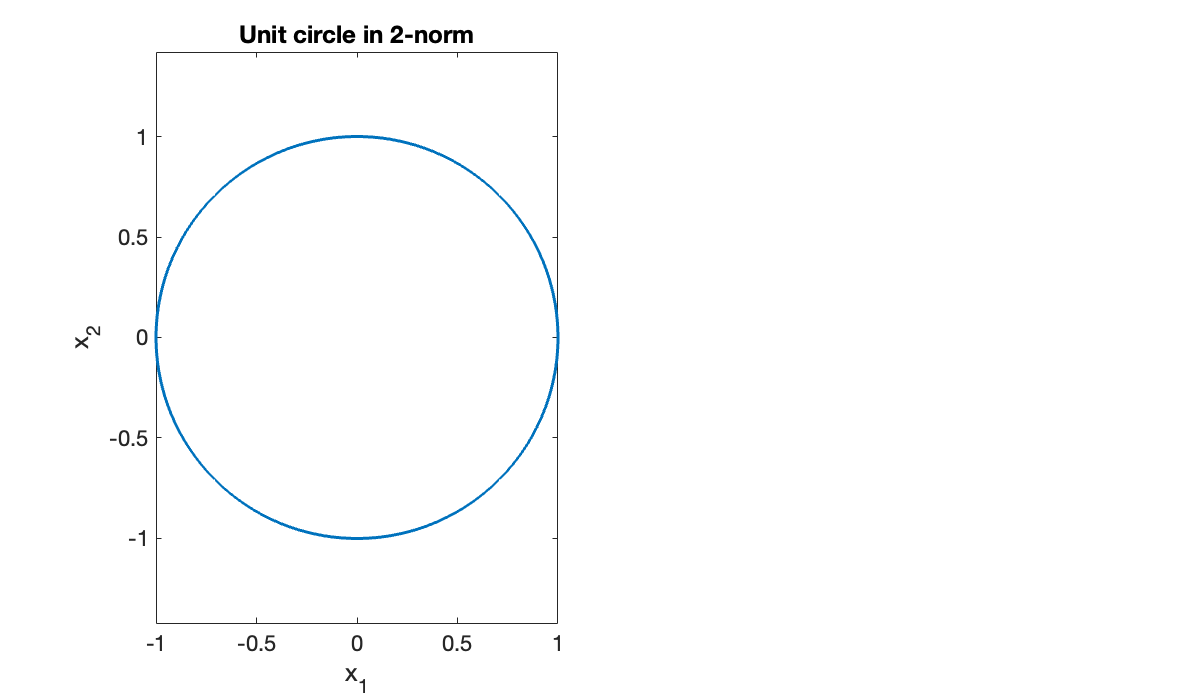
The linear function defines a mapping from to . We can apply A to every column of x by using a single matrix multiplication.
Ax = A * x;The image of the transformed vectors is an ellipse that just touches the circle of radius :
subplot(1,2,2), plot(Ax(1,:), Ax(2,:)), axis equal
hold on, plot(twonorm * x(1,:), twonorm * x(2,:), '--')
title('Image of Ax, with ||A||')
xlabel('x_1')
ylabel(('x_2'));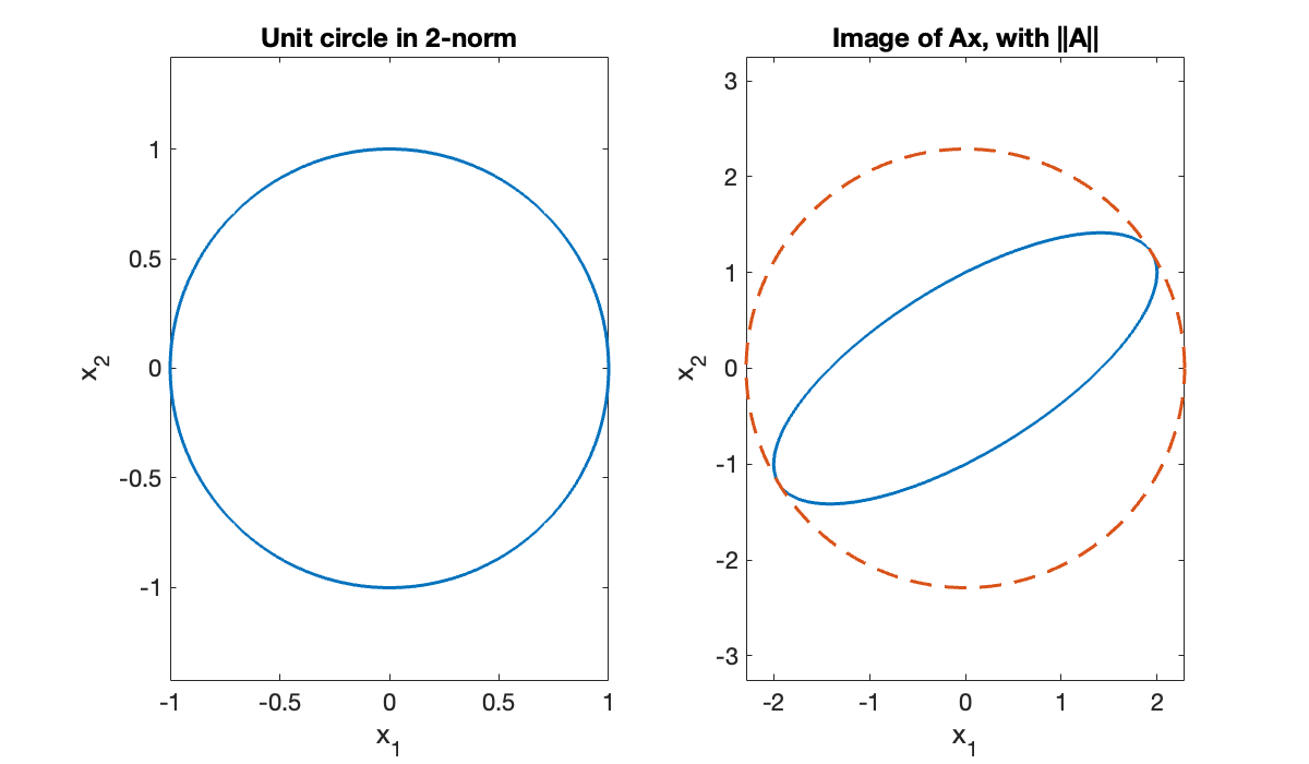
2.8 Conditioning of linear systems
Example 2.8.1
MATLAB has a function cond to compute matrix condition numbers. By default, the 2-norm is used. As an example, the family of Hilbert matrices is famously badly conditioned. Here is the case.
A = hilb(6)
kappa = cond(A)Because , it’s possible to lose nearly 8 digits of accuracy in the process of passing from and to . That fact is independent of the algorithm; it’s inevitable once the data are expressed in finite precision.
Let’s engineer a linear system problem to observe the effect of a perturbation. We will make sure we know the exact answer.
x = (1:6)';
b = A * x;
Now we perturb the system matrix and vector randomly by 10-10 in norm.
dA = randn(size(A));  dA = 1e-10 * (dA / norm(dA));
db = randn(size(b));  db = 1e-10 * (db / norm(db));
We solve the perturbed problem using pivoted LU and see how the solution was changed.
new_x = ((A + dA) \ (b + db));
dx = new_x - x;
Here is the relative error in the solution.
relative_error = norm(dx) / norm(x)And here are upper bounds predicted using the condition number of the original matrix.
upper_bound_b = (kappa * norm(db) / norm(b))
upper_bound_A = (kappa * norm(dA) / norm(A))Even if we didn’t make any manual perturbations to the data, machine roundoff does so at the relative level of .
dx = A\b - x;
relative_error = norm(dx) / norm(x)
rounding_bound = kappa * epsLarger Hilbert matrices are even more poorly conditioned:
A = hilb(14);
kappa = cond(A)Note that κ exceeds . In principle we therefore may end up with an answer that has relative error greater than 100%.
rounding_bound = kappa * epsLet’s put that prediction to the test.
x = (1:14)';  b = A * x;
dx = A\b - x;
relative_error = norm(dx) / norm(x)As anticipated, the solution has zero accurate digits in the 2-norm.
2.9 Exploiting matrix structure
Example 2.9.1
Here is a small tridiagonal matrix. Note that there is one fewer element on the super- and subdiagonals than on the main diagonal.
A = [ 2 -1  0  0  0  0
      4  2 -1  0  0  0
      0  3  0 -1  0  0
      0  0  2  2 -1  0
      0  0  0  1  1 -1
      0  0  0  0  0  2 ];
We can extract the elements on any diagonal using the diag function. The main or central diagonal is numbered zero, above and to the right of that is positive, and below and to the left is negative.
Tip
The diag function extracts the elements from a specified diagonal of a matrix.
diag_main = diag(A, 0)'
diag_plusone = diag(A, 1)'
diag_minusone = diag(A,-1)'A = A + diag([5 8 6 7], 2)The lower and upper bandwidths of are repeated in the factors from the unpivoted LU factorization.
[L, U] = lufact(A)Example 2.9.2
We begin with a symmetric .
A_1 = [ 2     4     4     2
        4     5     8    -5
        4     8     6     2
        2    -5     2   -26 ];
We won’t use pivoting, so the pivot element is at position (1,1). This will become the first element on the diagonal of . Then we divide by that pivot to get the first column of .
L = eye(4);
d = zeros(4, 1);
d(1) = A_1(1, 1);
L(:, 1) = A_1(:, 1) / d(1);
A_2 = A_1 - d(1) * L(:, 1) * L(:, 1)'We are now set up the same way for the submatrix in rows and columns 2–4.
d(2) = A_2(2, 2);
L(:, 2) = A_2(:, 2) / d(2);
A_3 = A_2 - d(2) * L(:, 2) * L(:, 2)'We continue working our way down the diagonal.
d(3) = A_3(3, 3);
L(:, 3) = A_3(:, 3) / d(3);
A_4 = A_3 - d(3) * L(:, 3) * L(:, 3)'
d(4) = A_4(4, 4);
d
LWe have arrived at the desired factorization, which we can validate:
norm(A_1 - (L * diag(d) * L'))Example 2.9.3
A randomly chosen matrix is extremely unlikely to be symmetric. However, there is a simple way to symmetrize one.
A = magic(4) + eye(4);
B = A + A'Similarly, a random symmetric matrix is unlikely to be positive definite. The Cholesky algorithm always detects a non-PD matrix by quitting with an error.
Tip
The chol function computes a Cholesky factorization if possible, or throws an error for a non-positive-definite matrix.
chol(B) % throws an errorError using chol
Matrix must be positive definite.It’s not hard to manufacture an SPD matrix to try out the Cholesky factorization.
B = A' * A;
R = chol(B)Here we validate the factorization:
norm(R' * R - B) / norm(B)