Functions
Newton’s method
1 2 3 4 5 6 7 8 9 10 11 12 13 14 15 16 17 18 19 20 21 22 23 24 25 26 27 28 29function x = newton(f,dfdx,x1) % NEWTON Newton's method for a scalar equation. % Input: % f objective function % dfdx derivative function % x1 initial root approximation % Output % x vector of root approximations (last one is best) % Operating parameters. funtol = 100*eps; xtol = 100*eps; maxiter = 40; x = x1; y = f(x1); dx = Inf; % for initial pass below k = 1; while (abs(dx) > xtol) && (abs(y) > funtol) && (k < maxiter) dydx = dfdx(x(k)); dx = -y/dydx; % Newton step x(k+1) = x(k) + dx; k = k+1; y = f(x(k)); end if k==maxiter warning('Maximum number of iterations reached.') end
Secant method
1 2 3 4 5 6 7 8 9 10 11 12 13 14 15 16 17 18 19 20 21 22 23 24 25 26 27function x = secant(f,x1,x2) % SECANT Secant method for a scalar equation. % Input: % f objective function % x1,x2 initial root approximations % Output % x vector of root approximations (last is best) % Operating parameters. funtol = 100*eps; xtol = 100*eps; maxiter = 40; x = [x1 x2]; dx = Inf; y1 = f(x1); k = 2; y2 = f(x2); while (abs(dx) > xtol) && (abs(y2) > funtol) && (k < maxiter) dx = -y2 * (x(k)-x(k-1)) / (y2-y1); % secant step x(k+1) = x(k) + dx; k = k+1; y1 = y2; % current f-value becomes the old one next time y2 = f(x(k)); end if k==maxiter warning('Maximum number of iterations reached.') end
Newton’s method for systems
1 2 3 4 5 6 7 8 9 10 11 12 13 14 15 16 17 18 19 20 21 22 23 24 25 26 27function x = newtonsys(f,x1) % NEWTONSYS Newton's method for a system of equations. % Input: % f function that computes residual and Jacobian matrix % x1 initial root approximation (n-vector) % Output % x array of approximations (one per column, last is best) % Operating parameters. funtol = 1000*eps; xtol = 1000*eps; maxiter = 40; x = x1(:); [y,J] = f(x1); dx = Inf; k = 1; while (norm(dx) > xtol) && (norm(y) > funtol) && (k < maxiter) dx = -(J\y); % Newton step x(:,k+1) = x(:,k) + dx; k = k+1; [y,J] = f(x(:,k)); end if k==maxiter warning('Maximum number of iterations reached.') end
Finite differences for Jacobian
1 2 3 4 5 6 7 8 9 10 11 12 13 14 15 16function J = fdjac(f,x0,y0) % FDJAC Finite-difference approximation of a Jacobian. % Input: % f function to be differentiated % x0 evaluation point (n-vector) % y0 value of f at x0 (m-vector) % Output % J approximate Jacobian (m-by-n) delta = sqrt(eps); % FD step size m = length(y0); n = length(x0); J = zeros(m,n); I = eye(n); for j = 1:n J(:,j) = ( f(x0+delta*I(:,j)) - y0) / delta; end
Levenberg’s method
1 2 3 4 5 6 7 8 9 10 11 12 13 14 15 16 17 18 19 20 21 22 23 24 25 26 27 28 29 30 31 32 33 34 35 36 37 38 39 40 41 42 43 44 45 46 47 48 49 50 51 52function x = levenberg(f,x1,tol) % LEVENBERG Quasi-Newton method for nonlinear systems. % Input: % f objective function % x1 initial root approximation % tol stopping tolerance (default is 1e-12) % Output % x array of approximations (one per column) % Operating parameters. if nargin < 3, tol = 1e-12; end ftol = tol; xtol = tol; maxiter = 40; x = x1(:); fk = f(x1); k = 1; s = Inf; Ak = fdjac(f,x(:,1),fk); % start with FD Jacobian jac_is_new = true; I = eye(length(x)); lambda = 10; while (norm(s) > xtol) && (norm(fk) > ftol) && (k < maxiter) % Compute the proposed step. B = Ak'*Ak + lambda*I; z = Ak'*fk; s = -(B\z); xnew = x(:,k) + s; fnew = f(xnew); % Do we accept the result? if norm(fnew) < norm(fk) % accept y = fnew - fk; x(:,k+1) = xnew; fk = fnew; k = k+1; lambda = lambda/10; % get closer to Newton % Broyden update of the Jacobian. Ak = Ak + (y-Ak*s)*(s'/(s'*s)); jac_is_new = false; else % don't accept % Get closer to steepest descent. lambda = lambda*4; % Re-initialize the Jacobian if it's out of date. if ~jac_is_new Ak = fdjac(f,x(:,k),fk); jac_is_new = true; end end end if (norm(fk) > 1e-3) warning('Iteration did not find a root.') end
Examples
4.1 The rootfinding problem
Example 4.1.1
J3 = @(x) besselj(3,x);
fplot(J3, [0, 20])
grid on
xlabel('x'), ylabel('J_3(x)')
title('Bessel function')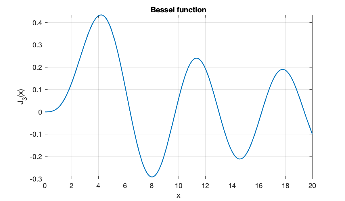
From the graph we see roots near 6, 10, 13, 16, and 19. We use nlsolve from the NLsolve package to find these roots accurately. It uses vector variables, so we have to code accordingly.
Tip
Type \omega followed by Tab to get the character ω.
The argument ftol=1e-14 below is called a keyword argument. Here it sets a goal for the maximum value of .
omega = [];
for guess = [6, 10, 13, 16, 19]
    omega = [omega; fzero(J3, guess)];
end
omegatable(omega, J3(omega), 'VariableNames', {'root estimate', 'function value'})hold on
scatter(omega, J3(omega))
title('Bessel roots')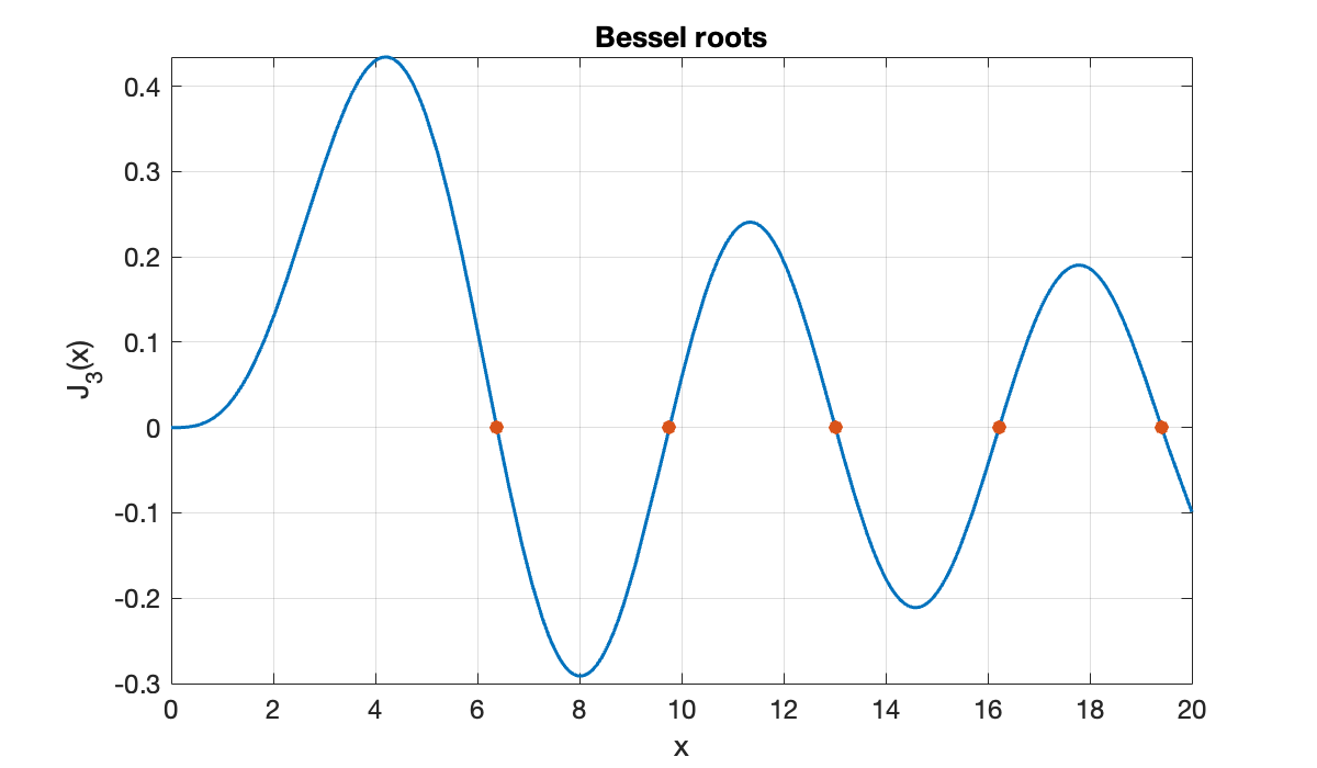
If instead we seek values at which , then we must find roots of the function .
omega = [];
for guess = [3, 6, 10, 13]
    f = @(x) J3(x) - 0.2;
    omega = [omega; fzero(f, guess)];
end
scatter(omega, J3(omega), '<')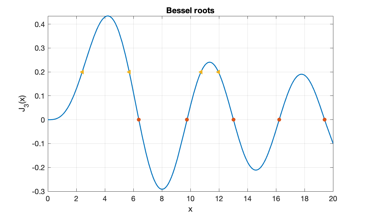
Example 4.1.2
Consider first the function
f = @(x) (x - 1) .* (x - 2);At the root , we have . If the values of were perturbed at every point by a small amount of noise, we can imagine finding the root of the function drawn with a thick ribbon, giving a range of potential roots.
clf
interval = [0.8, 1.2];
fplot(f, interval)
grid on, hold on
fplot(@(x) f(x) + 0.02, interval, 'k')
fplot(@(x) f(x) - 0.02, interval, 'k')
axis equal,  yticks([0])
ylim([-0.1, 0.1])
xlabel('x'), ylabel('f(x)')
title('Well-conditioned root')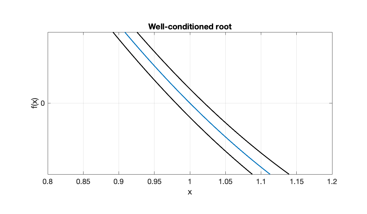
The possible values for a perturbed root all lie within the interval where the ribbon intersects the -axis. The width of that zone is about the same as the vertical thickness of the ribbon.
By contrast, consider the function
f = @(x) (x - 1) .* (x - 1.01);Now , and the graph of will be much shallower near . Look at the effect this has on our thick rendering:
axis(axis), cla
fplot(f, interval)
fplot(@(x) f(x) + 0.02, interval, 'k')
fplot(@(x) f(x) - 0.02, interval, 'k')
ylim([-0.1, 0.1]), yticks([0])
title('Poorly conditioned root')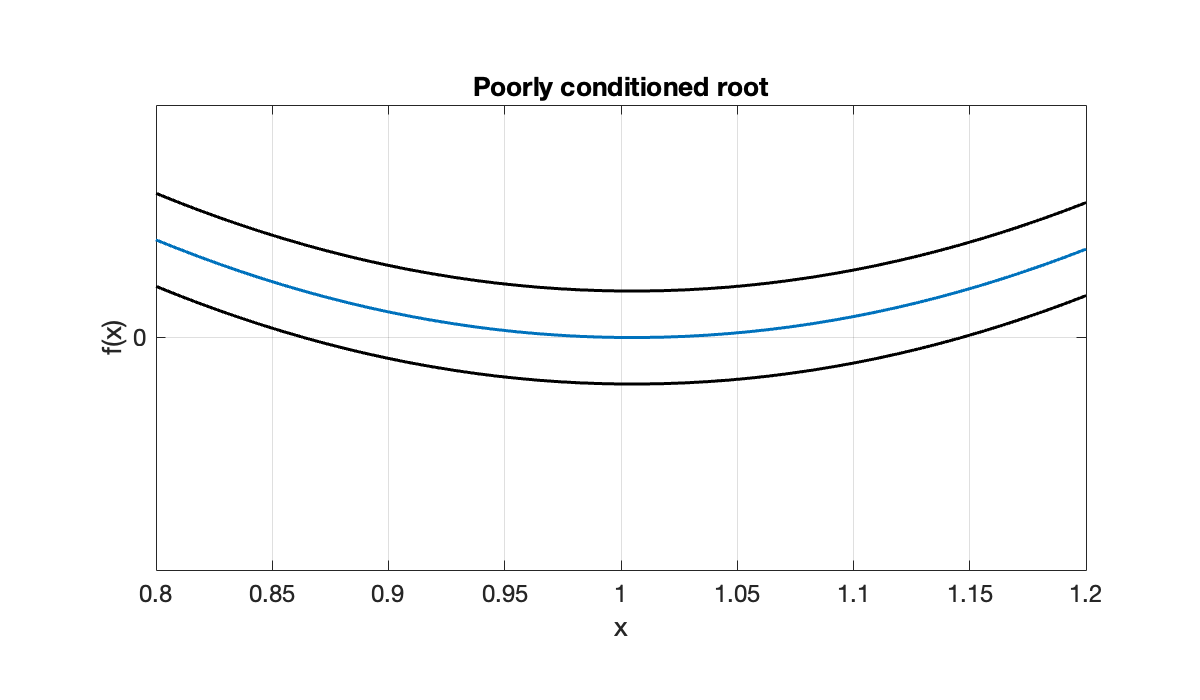
The vertical displacements in this picture are exactly the same as before. But the potential horizontal displacement of the root is much wider. In fact, if we perturb the function entirely upward by the amount drawn here, the root disappears!
4.2 Fixed-point iteration
Example 4.2.1
Let’s convert the roots of a quadratic polynomial to a fixed point problem.
f = @(x) x.^2 - 4*x + 3.5;
r = roots([1, -4, 3.5])We define .
g = @(x) x - f(x);Intersections of with the line are fixed points of and thus roots of . (Only one is shown in the chosen plot range.)
clf
fplot(g, [2, 3])
hold on,  plot([2, 3], [2, 3], 'k')
title('Finding a fixed point'),  axis equal
xlabel('x'),  ylabel('y')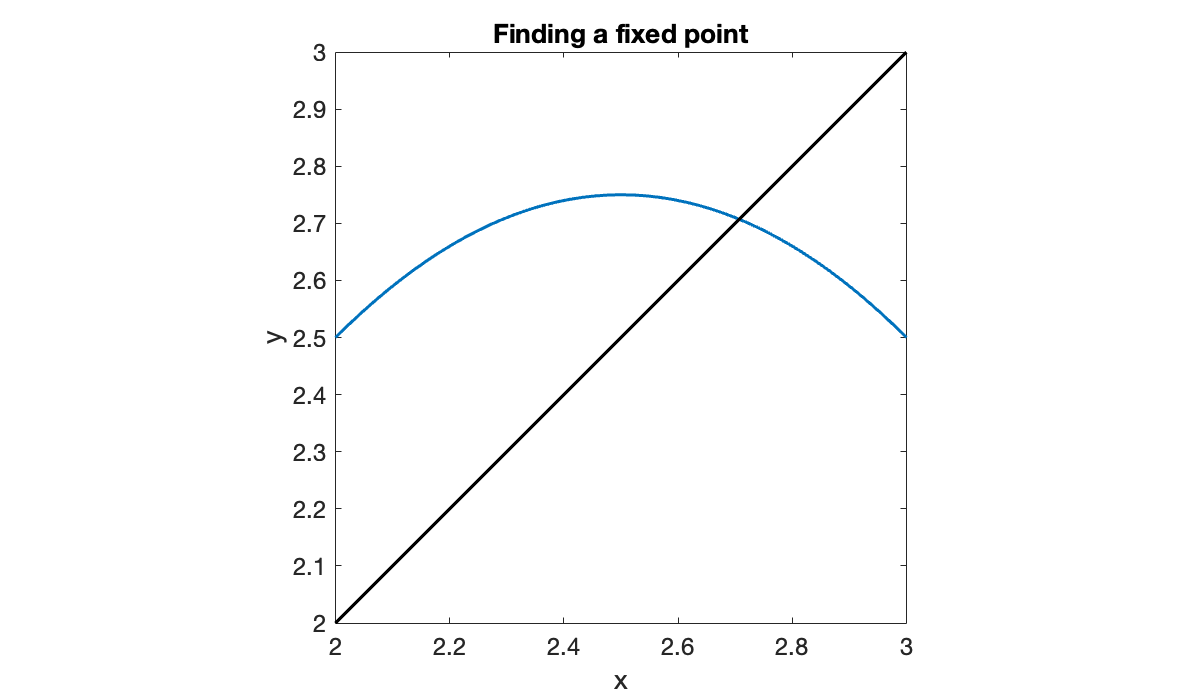
If we evaluate , we get a value of almost 2.6, so this is not a fixed point.
x = 2.1;
y = g(x)However, is considerably closer to the fixed point at around 2.7 than is. Suppose then that we adopt as our new value. Changing the coordinate in this way is the same as following a horizontal line over to the graph of .
plot([x, y], [y, y], '-')
x = y;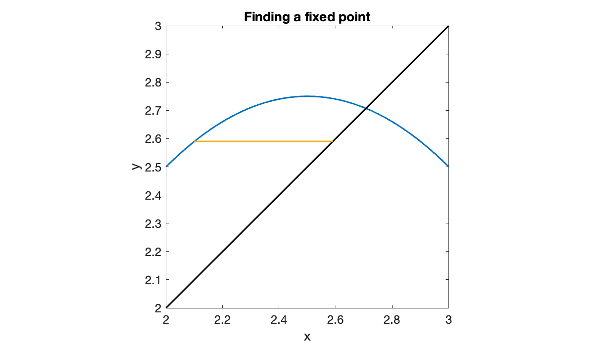
Now we can compute a new value for . We leave alone here, so we travel along a vertical line to the graph of .
y = g(x)
plot([x, x],[x, y], '-')You see that we are in a position to repeat these steps as often as we like. Let’s apply them a few times and see the result.
for k = 1:5
    plot([x, y], [y, y], '-')
    x = y;       % y --> new x
    y = g(x);    % g(x) --> new y
    plot([x, x], [x, y], '-')
end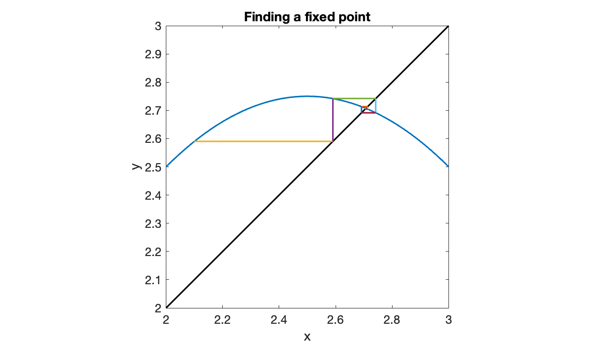
The process spirals in beautifully toward the fixed point we seek. Our last estimate has almost 4 accurate digits.
abs(y - r(1)) / r(1)Now let’s try to find the other fixed point in the same way. We’ll use 1.3 as a starting approximation.
cla
fplot(g, [1, 2])
hold on, plot([1, 2], [1, 2], 'k')
ylim([1, 2])
x = 1.3;  y = g(x);
for k = 1:5
    plot([x, y], [y, y], '-'),
    x = y;       % y --> new x
    y = g(x);    % g(x) --> new y
    plot([x, x], [x, y], '-')
end
title('No convergence')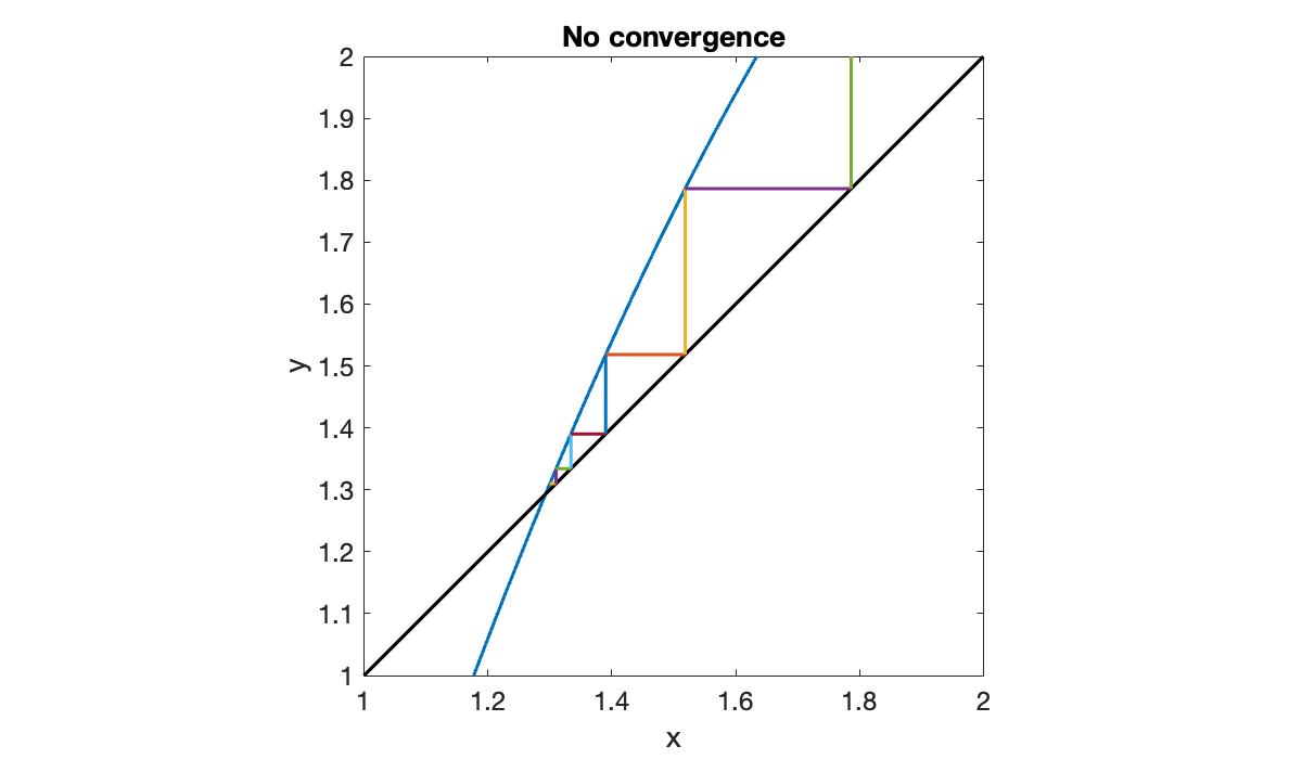
This time, the iteration is pushing us away from the correct answer.
Example 4.2.3
We revisit Demo 4.2.1 and investigate the observed convergence more closely. Recall that above we calculated at the convergent fixed point.
f = @(x) x.^2 - 4*x + 3.5;
r = roots([1, -4, 3.5]);
Here is the fixed-point iteration. This time we keep track of the whole sequence of approximations.
g = @(x) x - f(x);
x = 2.1;
for k = 1:12
    x(k+1) = g(x(k));
end
It’s illuminating to construct and plot the sequence of errors.
err = abs(x - r(1));
clf
semilogy(err, 'o-'), axis tight
xlabel('iteration'),  ylabel('error')
title('Convergence of fixed-point iteration')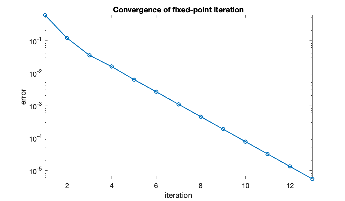
It’s quite clear that the convergence quickly settles into a linear rate. We could estimate this rate by doing a least-squares fit to a straight line. Keep in mind that the values for small should be left out of the computation, as they don’t represent the linear trend.
y = log(err(5:12));
p = polyfit(5:12, y, 1);
We can exponentiate the slope to get the convergence constant σ.
sigma = exp(p(1))The error should therefore decrease by a factor of σ at each iteration. We can check this easily from the observed data.
err(9:12) ./ err(8:11)The methods for finding σ agree well.
4.3 Newton’s method
Example 4.3.1
Suppose we want to find a root of the function
f = @(x) x .* exp(x) - 2;
clf, fplot(f, [0, 1.5])
xlabel('x'), ylabel('y')
set(gca, 'ygrid', 'on')
title('Objective function')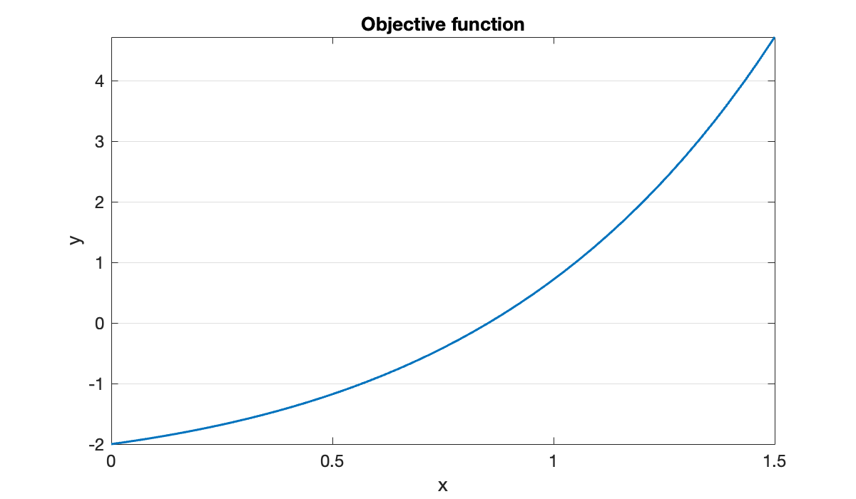
From the graph, it is clear that there is a root near . So we call that our initial guess, .
x1 = 1;
y1 = f(x1)
hold on, scatter(x1, y1, 'k')Next, we can compute the tangent line at the point , using the derivative.
df_dx = @(x) exp(x) .* (x + 1);
slope1 = df_dx(x1);
tangent1 = @(x) y1 + slope1 * (x - x1);
axis(axis)
fplot(tangent1, [0, 1.5], 'k--')
title('Function and tangent line')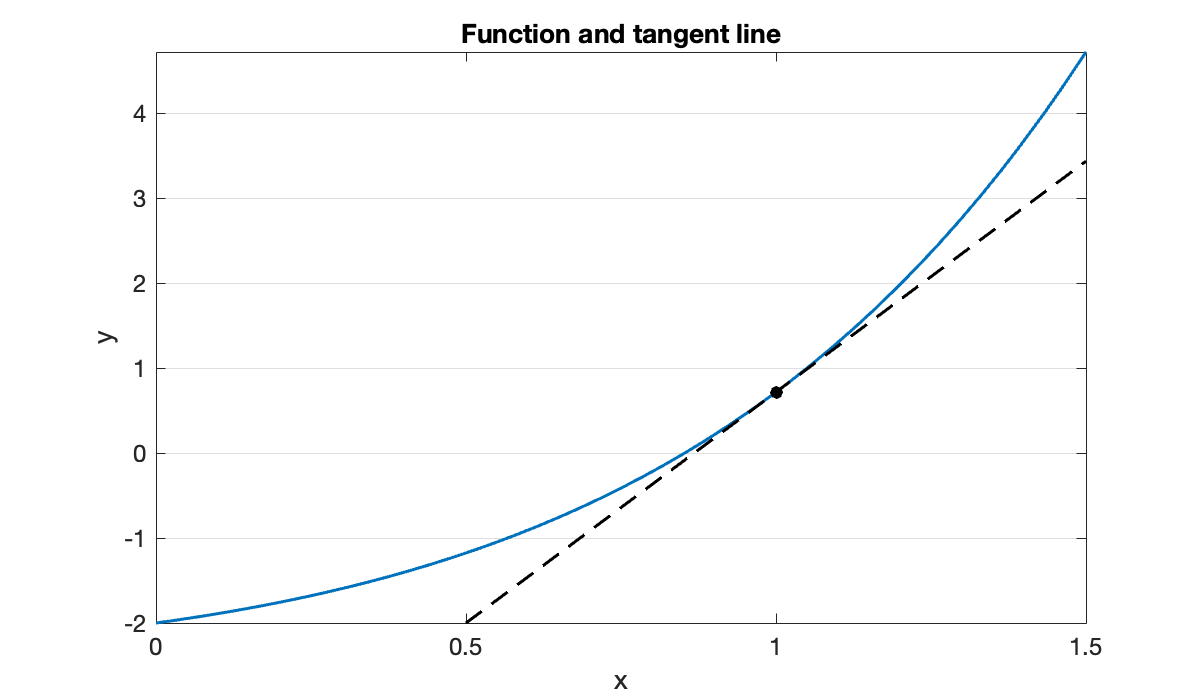
In lieu of finding the root of itself, we settle for finding the root of the tangent line approximation, which is trivial. Call this , our next approximation to the root.
x2 = x1 - y1 / slope1
scatter(x2, 0, 'r')
title('Root of the tangent')y2 = f(x2)The residual (i.e., value of ) is smaller than before, but not zero. So we repeat the process with a new tangent line based on the latest point on the curve.
cla,  axis auto
fplot(f, [0.83, 0.88])
scatter(x2, y2, 'k')
slope2 = df_dx(x2);
tangent2 = @(x) y2 + slope2 * (x - x2);
axis(axis)
fplot(tangent2, [0.8, 0.9], 'k--')
x3 = x2 - y2 / slope2;
scatter(x3, 0, 'r')
title('Next iteration')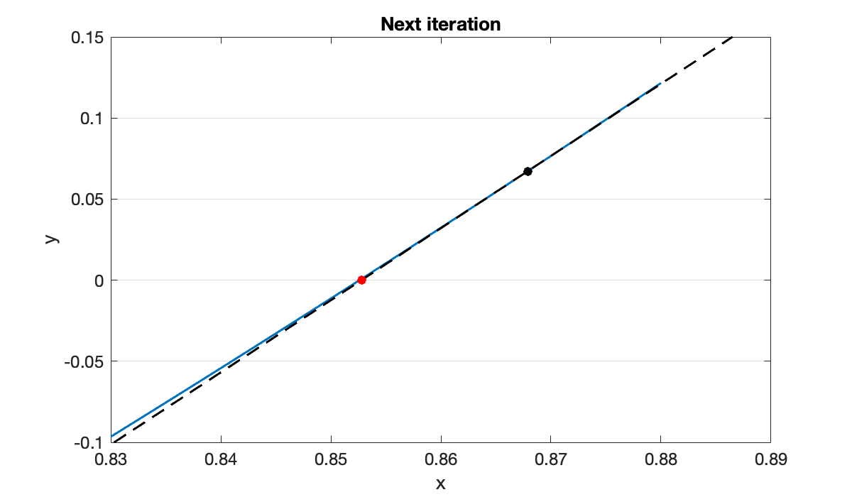
y3 = f(x3)Judging by the residual, we appear to be getting closer to the true root each time.
Example 4.3.2
We again look at finding a solution of near . To apply Newton’s method, we need to calculate values of both the residual function and its derivative.
f = @(x) x.*exp(x) - 2;
df_dx = @(x) exp(x).*(x+1);
We don’t know the exact root, so we use nlsolve to determine a proxy for it.
format long, r = fzero(f,1)We use as a starting guess and apply the iteration in a loop, storing the sequence of iterates in a vector.
x = 1;
for k = 1:6
    x(k+1) = x(k) - f(x(k)) / df_dx(x(k));
end
xHere is the sequence of errors.
format short e
err = x' - rThe exponents in the scientific notation definitely suggest a squaring sequence. We can check the evolution of the ratio in (4.3.9).
format short
logerr = log(abs(err))The clear convergence to 2 above constitutes good evidence of quadratic convergence.
Example 4.3.3
Suppose we want to evaluate the inverse of the function . This means solving for when is given, which has no elementary form. If a value of is given numerically, though, we simply have a rootfinding problem for .
Tip
When a function is created, it can refer to any variables in scope at that moment. Those values are locked in to the definition, which is called a closure. If the enclosed variables change values later, the function still uses the values it was created with.
h = @(x) exp(x) - x;
dh_dx = @(x) exp(x) - 1;
y_ = linspace(h(0), h(2), 200);
x_ = zeros(size(y_));
for i = 1:length(y_)
    f = @(x) h(x) - y_(i);
    df_dx = @(x) dh_dx(x);
    x = newton(f, df_dx, 1);  x_(i) = x(end);
end
clf, fplot(h, [0, 2])
hold on, axis equal
plot(y_, x_)
plot([0, max(y_)], [0, max(y_)], 'k--')
xlabel('x'), ylabel('y')
legend('h(x)', 'inverse', 'y=x');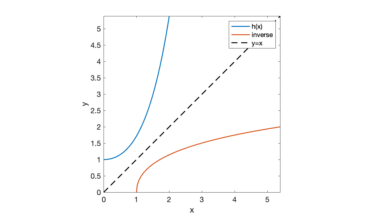
4.4 Interpolation-based methods
Example 4.4.1
We return to finding a root of the equation .
f = @(x) x .* exp(x) - 2;
clf, fplot(f, [0.25, 1.25])
set(gca, 'ygrid', 'on')
xlabel('x'), ylabel('y')
title('Objective function')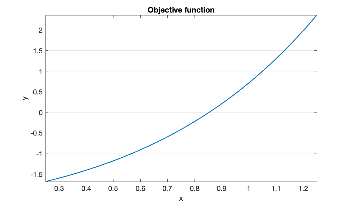
From the graph, it’s clear that there is a root near . To be more precise, there is a root in the interval . So let us take the endpoints of that interval as two initial approximations.
x1 = 1;    y1 = f(x1);
x2 = 0.5;  y2 = f(x2);
hold on, scatter([x1, x2], [y1, y2])
title('Two initial values')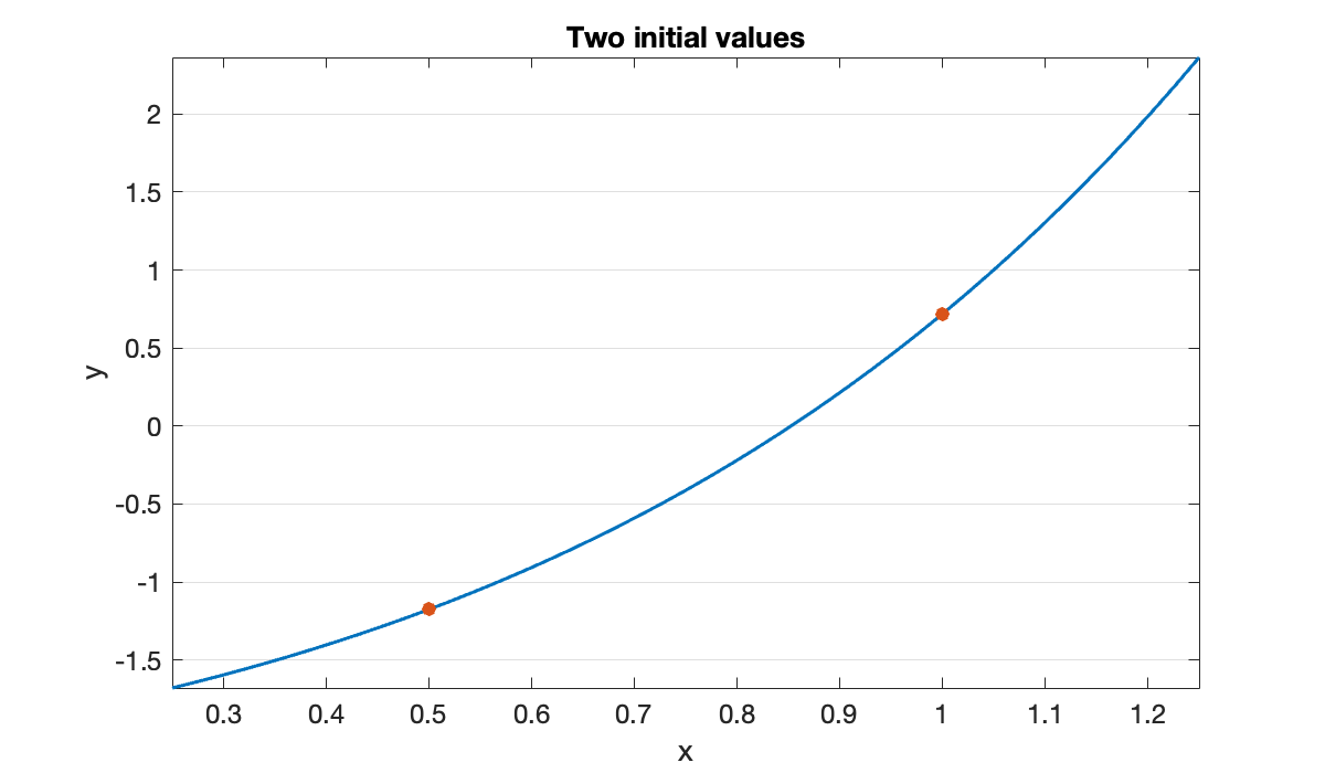
Instead of constructing the tangent line by evaluating the derivative, we can construct a linear model function by drawing the line between the two points and . This is called a secant line.
slope2 = (y2 - y1) / (x2 - x1);
secant2 = @(x) y2 + slope2 * (x - x2);
As before, the next root estimate in the iteration is the root of this linear model.
fplot(secant2,[0.25, 1.25],'k--')
x3 = x2 - y2 / slope2;
y3 = f(x3)
scatter(x3, 0)
title('Next value')For the next linear model, we use the line through the two most recent points. The next iterate is the root of that secant line, and so on.
slope2 = (y3 - y2) / (x3 - x2);
x4 = x3 - y3 / slope2;
y4 = f(x4)Example 4.4.2
We check the convergence of the secant method from Demo 4.4.1.
f = @(x) x .* exp(x) - 2;
x = secant(f, 1, 0.5);
We don’t know the exact root, so we use fzero to get a good proxy.
r = fzero(f, 1);Here is the sequence of errors.
format short e
err = r - x(1:end-1)'It’s not easy to see the convergence rate by staring at these numbers. We can use (4.4.8) to try to expose the superlinear convergence rate.
logerr = log(abs(err));
ratios = logerr(2:end) ./ logerr(1:end-1)As expected, this settles in at around 1.618.
Example 4.4.3
Here we look for a root of that is close to 1.
f = @(x) x + cos(10 * x);
interval = [0.5, 1.5];
clf, fplot(f, interval)
set(gca, 'ygrid', 'on'), axis(axis)
title('Objective function')
xlabel('x'), ylabel('y')
r = fzero(f, 1)We choose three values to get the iteration started.
x = [0.8, 1.2, 1]';
y = f(x);
hold on, scatter(x, y)
title('Three initial points')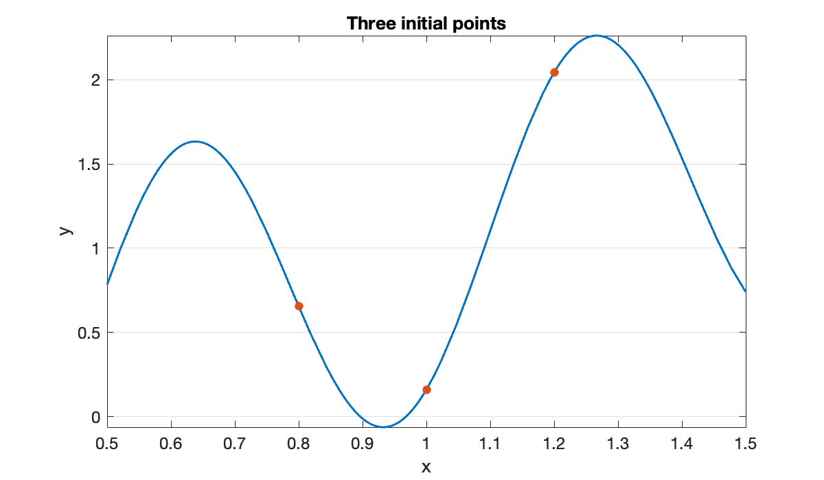
If we were using forward interpolation, we would ask for the polynomial interpolant of as a function of . But that parabola has no real roots.
c = polyfit(x, y, 2);    % coefficients of interpolant
q = @(x) polyval(c, x);
fplot(q, interval, '--')
title('Parabola model')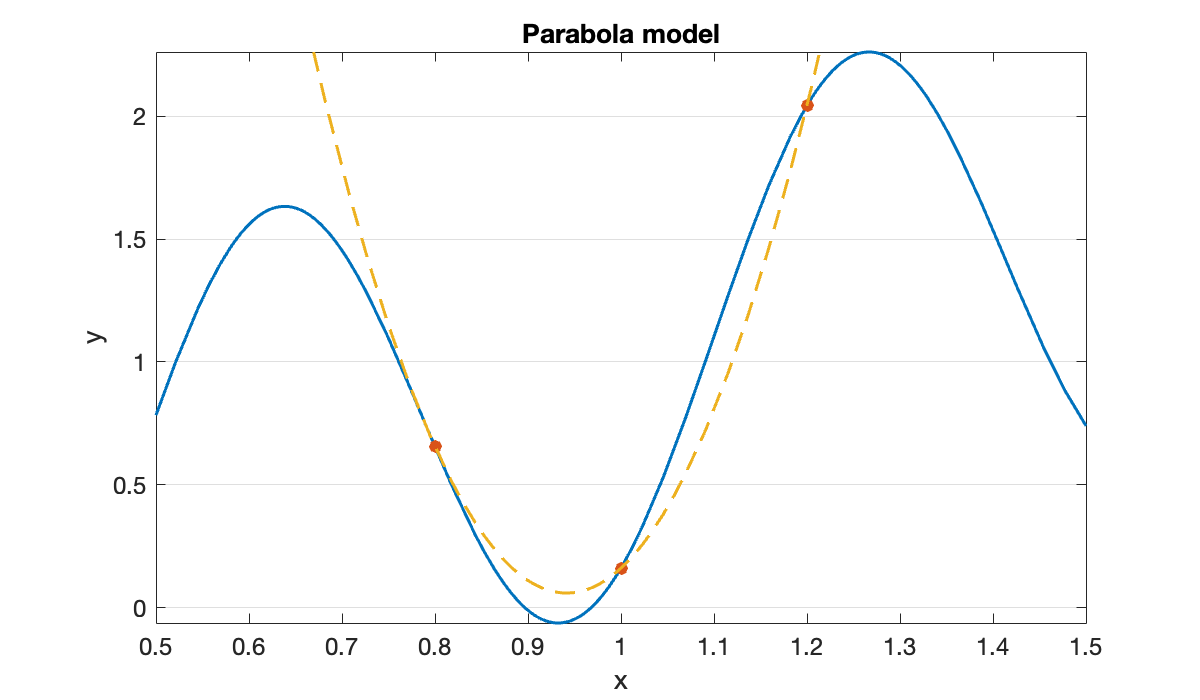
To do inverse interpolation, we swap the roles of and in the interpolation.
Tip
By giving two functions in the fplot call, we get the parametric plot as a function of .
cla, fplot(f, interval)
scatter(x, y)
c = polyfit(y, x, 2);    % coefficients of interpolating polynomial
q = @(y) polyval(c, y);
fplot(q, @(y) y, ylim,'--')    % plot x=q(y), y=y
title('Sideways parabola')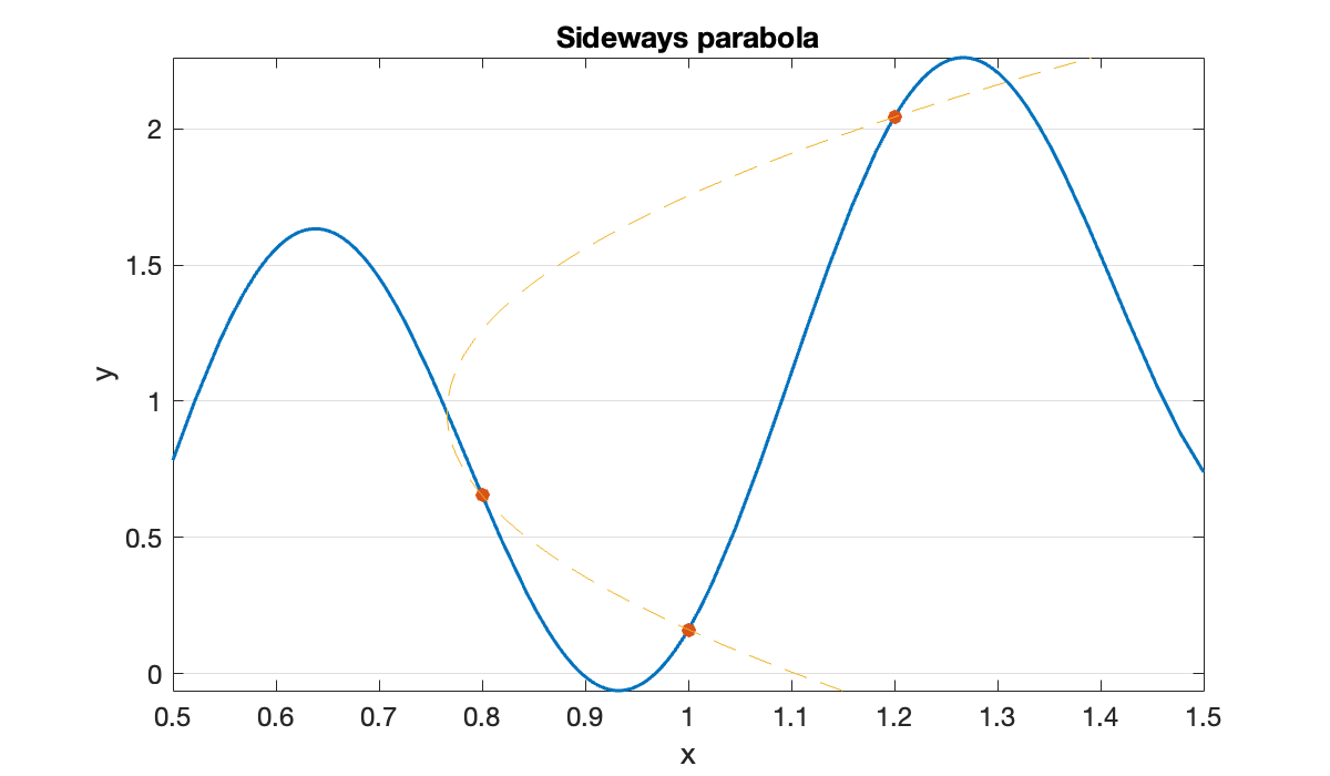
We seek the value of that makes zero. This means evaluating at zero.
x = [x; q(0)];
y = [y; f(x(end))]We repeat the process a few more times.
for k = 4:8
    c = polyfit(y(k-2:k), x(k-2:k), 2);
    x(k+1) = polyval(c, 0);
    y(k+1) = f(x(k+1));
end
disp('final residual:')
y(end)Here is the sequence of errors.
format short e
err = x - rThe convergence is probably superlinear:
logerr = log(abs(err));
ratios = logerr(2:end) ./ logerr(1:end-1)4.5 Newton for nonlinear systems
Example 4.5.3
A system of nonlinear equations is defined by its residual and Jacobian.
Tip
This function needs to be defined within a script file or in a file of its own with the .m extension.
function [f, J] = nlsystem(x)
    f = zeros(3, 1);   % ensure a column vector output
    f(1) = exp(x(2) - x(1)) - 2;
    f(2) = x(1) * x(2) + x(3);
    f(3) = x(2) * x(3) + x(1)^2 - x(2);
    J(1, :) = [-exp(x(2) - x(1)), exp(x(2) - x(1)), 0];
    J(2, :) = [x(2), x(1), 1];
    J(3, :) = [2 * x(1), x(3)-1, x(2)];
end
Since our system function is defined in an external file here, we need to use @ in order to reference it as a function argument.
nlsystem = @f45_nlsystem;
x1 = [0; 0; 0];    % column vector!
x = newtonsys(nlsystem, x1);
num_iter = size(x, 2)Let’s compute the residual of the last result in order to check the quality.
r = x(:, end)
back_err = norm(nlsystem(r))We take the sequence errors in the first component of the solution, applying the log so that we can look at the exponents.
log10( abs(x(1, 1:end-1) - r(1)) )'This sequence looks to be nearly doubling at each iteration, which is a good sign of quadratic convergence.
4.6 Quasi-Newton methods
Example 4.6.1
To solve a nonlinear system, we need to code only the function defining the system, and not its Jacobian.
Tip
A rule of thumb is that if you use a function as an input argument for another function, there needs to be an @ involved once: either for an anonymous definition or to reference a function defined elsewhere.
function [f, J] = nlsystem(x)
    f = zeros(3, 1);   % ensure a column vector output
    f(1) = exp(x(2) - x(1)) - 2;
    f(2) = x(1) * x(2) + x(3);
    f(3) = x(2) * x(3) + x(1)^2 - x(2);
    J(1, :) = [-exp(x(2) - x(1)), exp(x(2) - x(1)), 0];
    J(2, :) = [x(2), x(1), 1];
    J(3, :) = [2 * x(1), x(3)-1, x(2)];
end
In all other respects usage is the same as for the newtonsys function.
f = @f46_nlsystem;
x1 = [0; 0; 0];
x = levenberg(f, x1);
It’s always a good idea to check the accuracy of the root, by measuring the residual (backward error).
r = x(:, end)
backward_err = norm(f(r))Looking at the convergence of the first component, we find a rate between linear and quadratic, like with the secant method.
log10( abs(x(1, 1:end-1) - r(1)) )'4.7 Nonlinear least squares
Example 4.7.1
We will observe the convergence of Function 4.6.3 for different levels of the minimum least-squares residual. We start with a function mapping from into , and a point that will be near the optimum.
g = @(x) [sin(x(1) + x(2)); cos(x(1) - x(2)); exp(x(1) - x(2))];
p = [1; 1];
The function obviously has a zero residual at . We’ll make different perturbations of that function in order to create nonzero residuals.
Tip
@sprintf is a way to format numerical values as strings, patterned after the C function printf.
clf
labels = [];
for R = [1e-3, 1e-2, 1e-1]
    % Define the perturbed function.
    f = @(x) g(x) - g(p) + R * [-1; 1; -1] / sqrt(3)
    x = levenberg(f, [0; 0]);
    r = x(:, end);
    err = abs(x(1, 1:end-1) - r(1));
    normres = norm(f(r));
    semilogy(err), hold on
    labels = [labels; sprintf("R=%.2g", normres)];
end
xlabel("iteration"), ylabel("error")
legend(labels);In the least perturbed case, where the minimized residual is less than 10-3, the convergence is plausibly quadratic. At the next level up, the convergence starts similarly but suddenly stagnates for a long time. In the most perturbed case, the quadratic phase is nearly gone and the overall shape looks linear.
Example 4.7.2
m = 25; V = 2; Km = 0.5;
s = linspace(0.05, 6, m)';
w = V * s ./ (Km + s);                      % exactly on the curve
w = w + 0.15 * cos(2 * exp(s / 16) .* s);   % noise added
clf, fplot(@(s) V * s ./ (Km + s), [0, 6], '--')
hold on, scatter(s, w)
xlabel('concentration'), ylabel('reaction rate')
labels = ["ideal", "noisy data"];
legend(labels, 'location', 'east');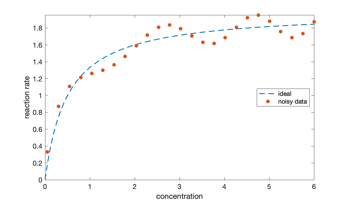
The idea is to pretend that we know nothing of the origins of this data and use nonlinear least squares to find the parameters in the theoretical model function . In (4.7.2), the variable plays the role of , and plays the role of . In the Jacobian, the derivatives are with respect to the parameters in .
function [f, J] = misfit(c, s, w)
    V = c(1);   Km = c(2);
    f = V * s ./ (Km + s) - w;
    J(:,1) = s ./ (Km + s);            % d/d(V)
    J(:,2) = -V * s ./ (Km + s).^2;    % d/d(Km)
end
The misfit function above has to know the parameters x that are being optimized as well as the data s and w that remain fixed. We use a closure to pass the data values along.
f = @(x) f47_misfit(x, s, w);Now we have a function that accepts a single 2-vector input and returns a 25-vector output. We can pass this function to levenberg to find the best-fit parameters.
x1 = [1; 0.75];
x = newtonsys(f, x1);
V = x(1, end),  Km = x(2, end)     % final values
model = @(s) V * s ./ (Km + s); % best-fit modelThe final values are reasonably close to the values , that we used to generate the noise-free data. Graphically, the model looks close to the original data:
final_misfit_norm = norm(model(s) - w)
hold on, fplot(model, [0, 6])
title('Michaelis-Menten fitting')
labels = [labels, "nonlinear fit"];
legend(labels, 'location', 'east');For this particular model, we also have the option of linearizing the fit process. Rewrite the model as
for the new fitting parameters and . This corresponds to the misfit function whose entries are
for . Although this misfit is nonlinear in and , it’s linear in the unknown parameters α and β. This lets us pose and solve it as a linear least-squares problem.
u = 1 ./ w;
A = [s.^(-1), s.^0];
z = A \ u;
alpha = z(1);  beta = z(2);
The two fits are different because they do not optimize the same quantities.
linmodel = @(s) 1 ./ (beta + alpha ./ s);
final_misfit_linearized = norm(linmodel(s) - w)
fplot(linmodel, [0, 6])
labels = [labels, "linearized fit"];
legend(labels, 'location', 'east');The truly nonlinear fit is clearly better in this case. It optimizes a residual for the original measured quantity rather than a transformed one we picked for algorithmic convenience.