Functions
Newton’s method
1 2 3 4 5 6 7 8 9 10 11 12 13 14 15 16 17 18 19 20 21 22 23 24 25 26 27 28 29 30 31def newton(f, dfdx, x1): """ newton(f, dfdx, x1) Use Newton's method to find a root of f starting from x1, where dfdx is the derivative of f. Returns a vector of root estimates. """ # Operating parameters. eps = np.finfo(float).eps funtol = 100 * eps xtol = 100 * eps maxiter = 40 x = np.zeros(maxiter) x[0] = x1 y = f(x1) dx = np.inf # for initial pass below k = 0 while (abs(dx) > xtol) and (abs(y) > funtol) and (k < maxiter): dydx = dfdx(x[k]) dx = -y / dydx # Newton step x[k + 1] = x[k] + dx # new estimate k = k + 1 y = f(x[k]) if k == maxiter: warnings.warn("Maximum number of iterations reached.") return x[:k+1]
About the code
Function 4.3.2 accepts keyword arguments. In the function declaration, these follow the semicolon, and when the function is called, they may be supplied as keyword=value in the argument list. Here, these arguments are also given default values by the assignments within the declaration. This arrangement is useful when there are multiple optional arguments, because the ordering of them doesn’t matter.
The break statement, seen here in line 25, causes an immediate exit from the innermost loop in which it is called. It is often used as a safety valve to escape an iteration that may not be able to terminate otherwise.
Secant method
1 2 3 4 5 6 7 8 9 10 11 12 13 14 15 16 17 18 19 20 21 22 23 24 25 26 27 28 29 30 31def secant(f, x1, x2): """ secant(f, x1, x2) Use the secant method to find a root of f starting from x1 and x2. Returns a vector of root estimates. """ # Operating parameters. eps = np.finfo(float).eps funtol = 100 * eps xtol = 100 * eps maxiter = 40 x = np.zeros(maxiter) x[:2] = [x1, x2] y1 = f(x1) y2 = 100 dx = np.inf # for initial pass below k = 1 while (abs(dx) > xtol) and (abs(y2) > funtol) and (k < maxiter): y2 = f(x[k]) dx = -y2 * (x[k] - x[k - 1]) / (y2 - y1) # secant step x[k + 1] = x[k] + dx # new estimate k = k + 1 y1 = y2 # current f-value becomes the old one next time if k == maxiter: warnings.warn("Maximum number of iterations reached.") return x[:k+1]
About the code
Because we want to observe the convergence of the method, Function 4.4.2 stores and returns the entire sequence of root estimates. However, only the most recent two are needed by the iterative formula. This is demonstrated by the use of y₁ and y₂ for the two most recent values of .
Newton’s method for systems
1 2 3 4 5 6 7 8 9 10 11 12 13 14 15 16 17 18 19 20 21 22 23 24 25 26 27 28 29def newtonsys(f, jac, x1): """ newtonsys(f, jac, x1) Use Newton's method to find a root of a system of equations, starting from x1. The function f should return the residual vector, and the function jac should return the Jacobian matrix. Returns root estimates as a matrix, one estimate per column. """ # Operating parameters. funtol = 1000 * np.finfo(float).eps xtol = 1000 * np.finfo(float).eps maxiter = 40 x = np.zeros((maxiter, len(x1))) x[0] = x1 y, J = f(x1), jac(x1) dx = 10.0 # for initial pass below k = 0 while (norm(dx) > xtol) and (norm(y) > funtol) and (k < maxiter): dx = -lstsq(J, y)[0] # Newton step x[k+1] = x[k] + dx k = k + 1 y, J = f(x[k]), jac(x[k]) if k == maxiter: warnings.warn("Maximum number of iterations reached.") return x[:k+1]
About the code
The output of Function 4.5.2 is a vector of vectors representing the entire history of root estimates. Since these should be in floating point, the starting value is converted with float before the iteration starts.
Finite differences for Jacobian
1 2 3 4 5 6 7 8 9 10 11 12 13 14 15def fdjac(f, x0, y0): """ fdjac(f,x0,y0) Compute a finite-difference approximation of the Jacobian matrix for f at x0, where y0=f(x0) is given. """ delta = np.sqrt(np.finfo(float).eps) # FD step size m, n = len(y0), len(x0) J = np.zeros((m, n)) I = np.eye(n) for j in range(n): J[:, j] = (f(x0 + delta * I[:, j]) - y0) / delta return J
About the code
Function 4.6.1 is written to accept the case where maps variables to values with , in anticipation of Nonlinear least squares.
Note that a default value is given for the third argument y₀, and it refers to earlier arguments in the list. The reason is that in some contexts, the caller of fdjac may have already computed y₀ and can supply it without computational cost, while in other contexts, it must be computed fresh. The configuration here adapts to either situation.
Levenberg’s method
1 2 3 4 5 6 7 8 9 10 11 12 13 14 15 16 17 18 19 20 21 22 23 24 25 26 27 28 29 30 31 32 33 34 35 36 37 38 39 40 41 42 43 44 45 46 47 48 49 50 51 52 53 54def levenberg(f, x1, tol=1e-12): """ levenberg(f,x1,tol) Use Levenberg's quasi-Newton iteration to find a root of the system f, starting from x1, with tol as the stopping tolerance in both step size and residual norm. Returns root estimates as a matrix, one estimate per column. """ # Operating parameters. ftol = tol xtol = tol maxiter = 40 n = len(x1) x = np.zeros((maxiter+1, n)) x[0] = x1 fk = f(x1) k = 0 s = 10.0 Ak = fdjac(f, x[0], fk) # start with FD Jacobian jac_is_new = True lam = 10 while (norm(s) > xtol) and (norm(fk) > ftol) and (k < maxiter): # Compute the proposed step. B = Ak.T @ Ak + lam * np.eye(n) z = Ak.T @ fk s = -lstsq(B, z)[0] xnew = x[k] + s fnew = f(xnew) # Do we accept the result? if norm(fnew) < norm(fk): # accept y = fnew - fk x[k + 1] = xnew fk = fnew k = k + 1 lam = lam / 10 # get closer to Newton # Broyden update of the Jacobian. Ak = Ak + np.outer(y - Ak @ s, s / np.dot(s, s)) jac_is_new = False else: # don't accept # Get closer to steepest descent. lam = lam * 4 # Re-initialize the Jacobian if it's out of date. if not jac_is_new: Ak = fdjac(f, x[k], fk) jac_is_new = True if norm(fk) > 1e-3: warnings.warn("Iteration did not find a root.") return x[:k+1]
Examples
4.1 The rootfinding problem
Example 4.1.1
import scipy.special as special
def J3(x):
    return special.jv(3.0, x)

xx = linspace(0, 20, 500)
fig, ax = subplots()
ax.plot(xx, J3(xx))
ax.grid()
xlabel("$x$"), ylabel("$J_3(x)$")
title("Bessel function");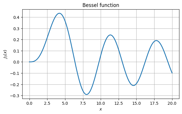
From the graph we see roots near 6, 10, 13, 16, and 19. We use root_scalar from the scipy.optimize package to find these roots accurately.
from scipy.optimize import root_scalar

omega = []
for guess in [6.0, 10.0, 13.0, 16.0, 19.0]:
    s = root_scalar(J3, bracket=[guess - 0.5, guess + 0.5]).root
    omega.append(s)

results = PrettyTable()
results.add_column("root estimate", omega)
results.add_column("function value", [J3(ω) for ω in omega])
print(results)
+--------------------+-------------------------+
| root estimate | function value |
+--------------------+-------------------------+
| 6.380161895923983 | 2.5877058405892666e-16 |
| 9.761023129981195 | -1.1824718824668837e-13 |
| 13.015200721698434 | -1.135864957485476e-16 |
| 16.223466160318758 | -1.898385896228919e-15 |
| 19.40941522643501 | 7.862906169587308e-16 |
+--------------------+-------------------------+
ax.scatter(omega, J3(omega))
ax.set_title("Bessel function roots")
fig
If instead we seek values at which , then we must find roots of the function .
omega = []
for guess in [3., 6., 10., 13.]:
    f = lambda x: J3(x) - 0.2
    s = root_scalar(f, x0=guess).root
    omega.append(s)

ax.scatter(omega, J3(omega))
fig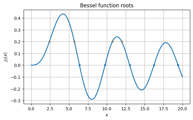
Example 4.1.2
Consider first the function
f = lambda x: (x - 1) * (x - 2)At the root , we have . If the values of were perturbed at every point by a small amount of noise, we can imagine finding the root of the function drawn with a thick ribbon, giving a range of potential roots.
xx = linspace(0.8, 1.2, 400)
plot(xx, f(xx))
plot(xx, f(xx) + 0.02, "k")
plot(xx, f(xx) - 0.02, "k")
axis("equal"), grid(True)
xlabel("x"), ylabel("f(x)")
title("Well-conditioned root");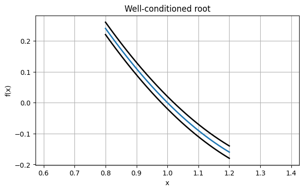
The possible values for a perturbed root all lie within the interval where the ribbon intersects the -axis. The width of that zone is about the same as the vertical thickness of the ribbon.
By contrast, consider the function
f = lambda x: (x - 1) * (x - 1.01)Now , and the graph of will be much shallower near . Look at the effect this has on our thick rendering:
xx = linspace(0.8, 1.2, 400)
plot(xx, f(xx))
plot(xx, f(xx) + 0.02, "k")
plot(xx, f(xx) - 0.02, "k")
axis("equal"), grid(True)
xlabel("x"), ylabel("f(x)")
title("Poorly-conditioned root");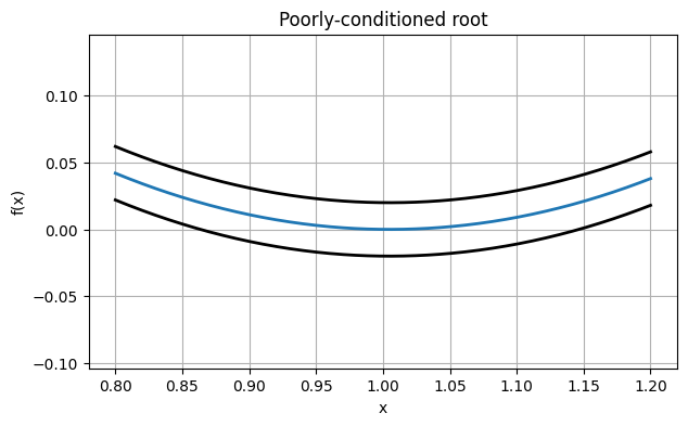
The vertical displacements in this picture are exactly the same as before. But the potential horizontal displacement of the root is much wider. In fact, if we perturb the function entirely upward by the amount drawn here, the root disappears!
4.2 Fixed-point iteration
Example 4.2.1
Let’s convert the roots of a quadratic polynomial to a fixed point problem.
f = poly1d([1, -4, 3.5])
r = f.roots
print(r)
[2.70710678 1.29289322]
We define .
g = lambda x: x - f(x)Intersections of with the line are fixed points of and thus roots of . (Only one is shown in the chosen plot range.)
fig, ax = subplots()
g = lambda x: x - f(x)
xx = linspace(2, 3, 400)
ax.plot(xx, g(xx), label="y=g(x)")
ax.plot(xx, xx, label="y=x")
axis("equal"), legend()
title("Finding a fixed point");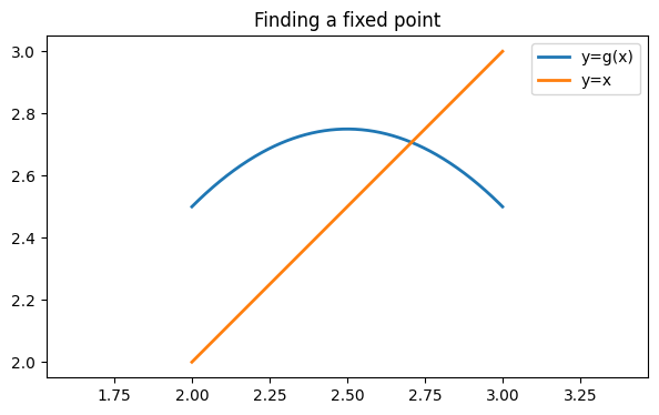
If we evaluate , we get a value of almost 2.6, so this is not a fixed point.
x = 2.1
y = g(x)
print(y)
2.59
However, is considerably closer to the fixed point at around 2.7 than is. Suppose then that we adopt as our new value. Changing the coordinate in this way is the same as following a horizontal line over to the graph of .
ax.plot([x, y], [y, y], "r:", label="")
fig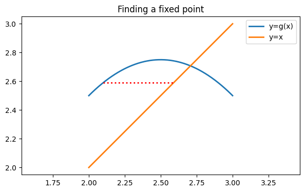
Now we can compute a new value for . We leave alone here, so we travel along a vertical line to the graph of .
x = y
y = g(x)
print("y:", y)
ax.plot([x, x], [x, y], "k:")
fig
y: 2.7419000000000002
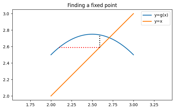
You see that we are in a position to repeat these steps as often as we like. Let’s apply them a few times and see the result.
for k in range(5):
    ax.plot([x, y], [y, y], "r:")
    x = y       # y --> new x
    y = g(x)    # g(x) --> new y
    ax.plot([x, x], [x, y], "k:")
fig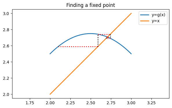
The process spirals in beautifully toward the fixed point we seek. Our last estimate has almost 4 accurate digits.
print(abs(y - max(r)) / max(r))0.0001653094344995643
Now let’s try to find the other fixed point in the same way. We’ll use 1.3 as a starting approximation.
xx = linspace(1, 2, 400)
fig, ax = subplots()
ax.plot(xx, g(xx), label="y=g(x)")
ax.plot(xx, xx, label="y=x")
ax.set_aspect(1.0)
ax.legend()

x = 1.3
y = g(x)
for k in range(5):
    ax.plot([x, y], [y, y], "r:")
    x = y
    y = g(x)
    ax.plot([x, x], [x, y], "k:")
ylim(1, 2.5)
title("No convergence");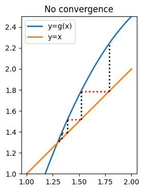
This time, the iteration is pushing us away from the correct answer.
Example 4.2.3
We revisit Demo 4.2.1 and investigate the observed convergence more closely. Recall that above we calculated at the convergent fixed point.
f = poly1d([1, -4, 3.5])
r = f.roots
print(r)
[2.70710678 1.29289322]
Here is the fixed-point iteration. This time we keep track of the whole sequence of approximations.
g = lambda x: x - f(x)
x = zeros(12)
x[0] = 2.1
for k in range(11):
    x[k + 1] = g(x[k])

print(x)
[2.1 2.59 2.7419 2.69148439 2.71333373 2.70448872
2.70818436 2.70665927 2.70729195 2.70703005 2.70713856 2.70709362]
It’s illuminating to construct and plot the sequence of errors.
err = abs(x - max(r))
semilogy(err, "-o")
xlabel("iteration number"), ylabel("error")
title("Convergence of fixed-point iteration");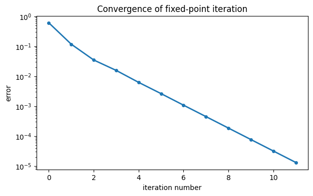
It’s quite clear that the convergence quickly settles into a linear rate. We could estimate this rate by doing a least-squares fit to a straight line. Keep in mind that the values for small should be left out of the computation, as they don’t represent the linear trend.
p = polyfit(arange(5, 13), log(err[4:]), 1)
print(p)
[-0.88071816 -0.66805739]
We can exponentiate the slope to get the convergence constant σ.
print("sigma:", exp(p[0]))sigma: 0.4144851385485472
The error should therefore decrease by a factor of σ at each iteration. We can check this easily from the observed data.
err[8:] / err[7:-1]array([0.41376605, 0.41439873, 0.41413683, 0.41424534])The methods for finding σ agree well.
4.3 Newton’s method
Example 4.3.1
Suppose we want to find a root of this function:
f = lambda x: x * exp(x) - 2
xx = linspace(0, 1.5, 400)

fig, ax = subplots()
ax.plot(xx, f(xx), label="function")
ax.grid()
ax.set_xlabel("$x$")
ax.set_ylabel("$y$");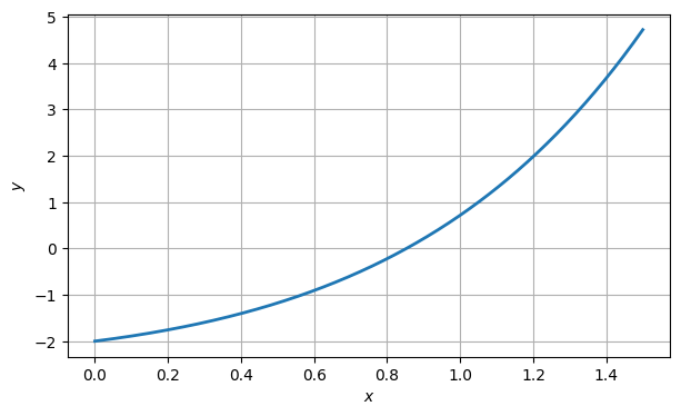
From the graph, it is clear that there is a root near . So we call that our initial guess, .
x1 = 1
y1 = f(x1)
ax.plot(x1, y1, "ko", label="initial point")
ax.legend()
fig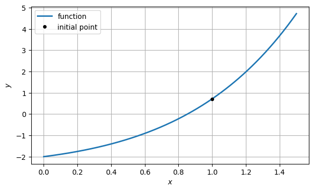
Next, we can compute the tangent line at the point , using the derivative.
df_dx = lambda x: exp(x) * (x + 1)
slope1 = df_dx(x1)
tangent1 = lambda x: y1 + slope1 * (x - x1)

ax.plot(xx, tangent1(xx), "--", label="tangent line")
ax.set_ylim(-2, 4)
ax.legend()
fig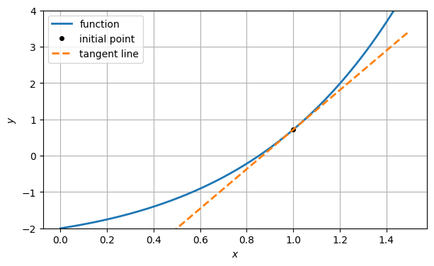
In lieu of finding the root of itself, we settle for finding the root of the tangent line approximation, which is trivial. Call this , our next approximation to the root.
x2 = x1 - y1 / slope1
ax.plot(x2, 0, "ko", label="tangent root")
ax.legend()
fig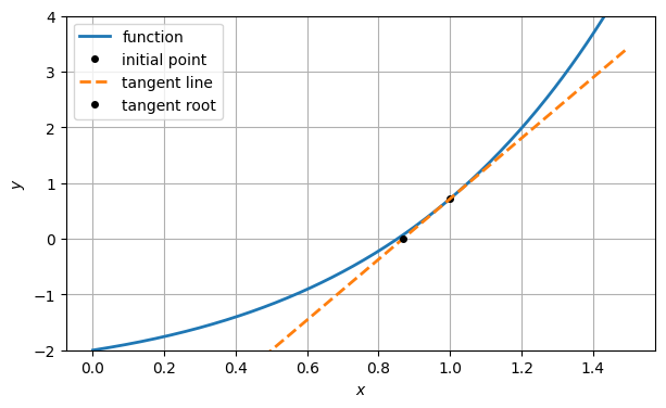
y2 = f(x2)
print(y2)
0.06716266657572145
The residual (i.e., value of ) is smaller than before, but not zero. So we repeat the process with a new tangent line based on the latest point on the curve.
xx = linspace(0.83, 0.88, 200)

plot(xx, f(xx))
plot(x2, y2, "ko")
grid(), xlabel("$x$"), ylabel("$y$")

slope2 = df_dx(x2)
tangent2 = lambda x: y2 + slope2 * (x - x2)
plot(xx, tangent2(xx), "--")
x3 = x2 - y2 / slope2
plot(x3, 0, "ko")
title("Second iteration");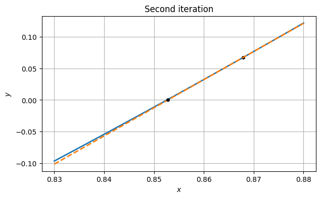
y3 = f(x3)
print(y3)
0.0007730906446230534
Judging by the residual, we appear to be getting closer to the true root each time.
Example 4.3.2
We again look at finding a solution of near . To apply Newton’s method, we need to calculate values of both the residual function and its derivative.
f = lambda x: x * exp(x) - 2
df_dx = lambda x: exp(x) * (x + 1)
We don’t know the exact root, so we use nlsolve to determine a proxy for it.
r = root_scalar(f, bracket=[0.8, 1.0]).root
print(r)
0.8526055020137255
We use as a starting guess and apply the iteration in a loop, storing the sequence of iterates in a vector.
x = ones(5)
for k in range(4):
    x[k + 1] = x[k] - f(x[k]) / df_dx(x[k])

print(x)
[1. 0.86787944 0.85278337 0.85260553 0.8526055 ]
Here is the sequence of errors.
err = x - r
print(err)
[1.47394498e-01 1.52739392e-02 1.77871403e-04 2.43551965e-08
4.44089210e-16]
The exponents in the scientific notation definitely suggest a squaring sequence. We can check the evolution of the ratio in (4.3.9).
logerr = log(abs(err))
for i in range(len(err) - 1):
    print(logerr[i+1] / logerr[i])
2.1840144823399648
2.064863881067786
2.030299689916648
2.01651205997716
The clear convergence to 2 above constitutes good evidence of quadratic convergence.
Example 4.3.3
Suppose we want to evaluate the inverse of the function . This means solving , or , for when is given. That equation has no solution in terms of elementary functions. If a value of is given numerically, though, we simply have a rootfinding problem for .
Tip
The enumerate function produces a pair of values for each iteration: a positional index and the corresponding contents.
h = lambda x: exp(x) - x
dh_dx = lambda x: exp(x) - 1
y_ = linspace(h(0), h(2), 200)
x_ = zeros(y_.shape)
for (i, y) in enumerate(y_):
    f = lambda x: h(x) - y
    df_dx = lambda x: dh_dx(x)
    x = FNC.newton(f, df_dx, y)
    x_[i] = x[-1]

plot(x_, y_, label="$y=h(x)$")
plot(y_, x_, label="$y=h^{-1}(x)$")
plot([0, max(y_)], [0, max(y_)], 'k--', label="")
title("Function and its inverse")
xlabel("x"), ylabel("y"), axis("equal")
ax.grid()
legend();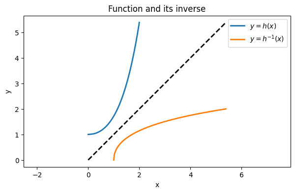
4.4 Interpolation-based methods
Example 4.4.1
f = lambda x: x * exp(x) - 2
xx = linspace(0.25, 1.25, 400)

fig, ax = subplots()
ax.plot(xx, f(xx), label="function")
ax.set_xlabel("$x$")
ax.set_ylabel("$f(x)$")
ax.grid();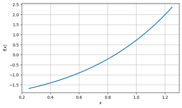
From the graph, it’s clear that there is a root near . To be more precise, there is a root in the interval . So let us take the endpoints of that interval as two initial approximations.
x1 = 1
y1 = f(x1)
x2 = 0.5
y2 = f(x2)
ax.plot([x1, x2], [y1, y2], "ko", label="initial points")
ax.legend()
fig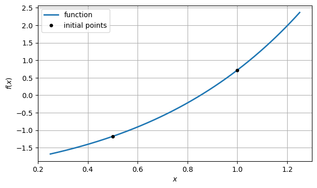
Instead of constructing the tangent line by evaluating the derivative, we can construct a linear model function by drawing the line between the two points and . This is called a secant line.
slope2 = (y2 - y1) / (x2 - x1)
secant2 = lambda x: y2 + slope2 * (x - x2)
ax.plot(xx, secant2(xx), "--", label="secant line")
ax.legend()
fig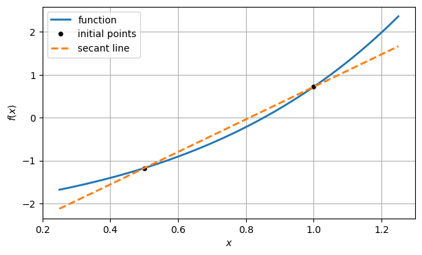
As before, the next root estimate in the iteration is the root of this linear model.
x3 = x2 - y2 / slope2
ax.plot(x3, 0, "o", label="root of secant")
y3 = f(x3)
print(y3)
ax.legend()
fig
-0.17768144843679456
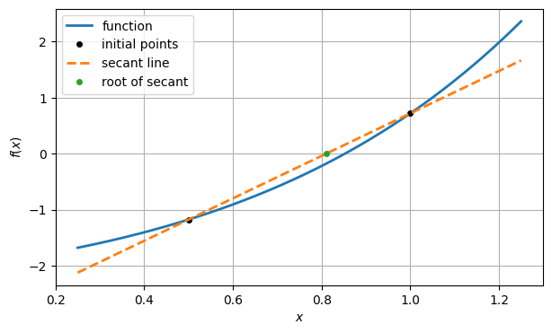
For the next linear model, we use the line through the two most recent points. The next iterate is the root of that secant line, and so on.
slope3 = (y3 - y2) / (x3 - x2)
x4 = x3 - y3 / slope3
print(f(x4))
0.05718067370113333
Example 4.4.2
We check the convergence of the secant method from Demo 4.4.1.
f = lambda x: x * exp(x) - 2
x = FNC.secant(f, 1, 0.5)
print(x)
[1. 0.5 0.81037177 0.86563193 0.85217802 0.85260123
0.8526055 0.8526055 0.8526055 ]
We don’t know the exact root, so we use root_scalar to get a substitute.
from scipy.optimize import root_scalar
r = root_scalar(f, bracket=[0.5, 1]).root
print(r)
0.8526055020137254
Here is the sequence of errors.
err = r - x
print(err)
[-1.47394498e-01 3.52605502e-01 4.22337271e-02 -1.30264253e-02
4.27479941e-04 4.26991559e-06 -1.40547707e-09 4.55191440e-15
0.00000000e+00]
It’s not easy to see the convergence rate by staring at these numbers. We can use (4.4.8) to try to expose the superlinear convergence rate.
logerr = log(abs(err))
for i in range(len(err) - 2):
    print(logerr[i+1] / logerr[i])
0.5444386280277934
3.0358017547194565
1.3716940021941457
1.7871469297607958
1.593780475055435
1.6485786717829443
1.62014464365765
/var/folders/gc/0752xrm56pnf0r0dsrn5370c0000gr/T/ipykernel_93663/1382054591.py:1: RuntimeWarning: divide by zero encountered in log
  logerr = log(abs(err))
As expected, this settles in at around 1.618.
Example 4.4.3
Here we look for a root of that is close to 1.
f = lambda x: x + cos(10 * x)
xx = linspace(0.5, 1.5, 400)
fig, ax = subplots()
ax.plot(xx, f(xx), label="function")
ax.grid()
xlabel("$x$"), ylabel("$y$")
fig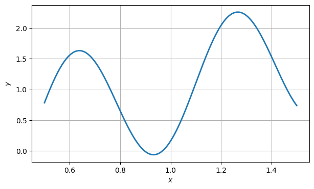

We choose three values to get the iteration started.
x = array([0.8, 1.2, 1])
y = f(x)
ax.plot(x, y, "ko", label="initial points")
ax.legend()
fig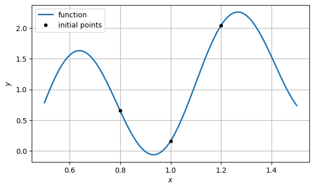
If we were using forward interpolation, we would ask for the polynomial interpolant of as a function of . But that parabola has no real roots.
q = poly1d(polyfit(x, y, 2))  # interpolating polynomial
ax.plot(xx, q(xx), "--", label="interpolant")
ax.set_ylim(-0.1, 3), ax.legend()
fig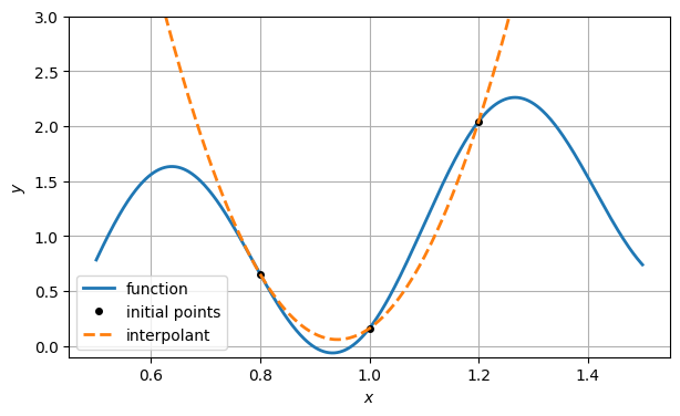
To do inverse interpolation, we swap the roles of and in the interpolation.
plot(xx, f(xx), label="function")
plot(x, y, "ko", label="initial points")

q = poly1d(polyfit(y, x, 2))  # inverse interpolating polynomial
yy = linspace(-0.1, 2.6, 400)
plot(q(yy), yy, "--", label="inverse interpolant")

grid(), xlabel("$x$"), ylabel("$y$")
legend();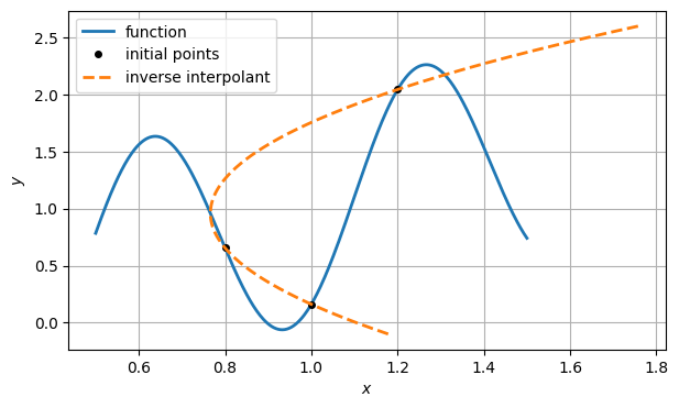
We seek the value of that makes zero. This means evaluating at zero.
x = hstack([x, q(0)])
y = hstack([y, f(x[-1])])
print("x:", x, "\ny:", y)
x: [0.8 1.2 1. 1.10398139]
y: [0.65449997 2.04385396 0.16092847 1.14820652]
We repeat the process a few more times.
for k in range(6):
    q = poly1d(polyfit(y[-3:], x[-3:], 2))
    x = hstack([x, q(0)])
    y = hstack([y, f(x[-1])])
print(f"final residual is {y[-1]:.2e}")
final residual is 1.53e-14
Here is the sequence of errors.
from scipy.optimize import root_scalar
r = root_scalar(f, bracket=[0.9, 1]).root
err = x - r
print(err)
[-1.67888402e-01 2.32111598e-01 3.21115982e-02 1.36092984e-01
1.53473435e-02 3.26831473e-03 4.61743614e-04 6.29584770e-06
3.43903683e-09 6.39488462e-14]
The error seems to be superlinear, but subquadratic:
logerr = log(abs(err))
for i in range(len(err) - 1):
    print(logerr[i+1] / logerr[i])
0.818477543986624
2.354297090262193
0.5800188694773638
2.0942526256501797
1.3702985897217315
1.341928284536791
1.5592238835564955
1.6273123235711273
1.5589376504302388
4.5 Newton for nonlinear systems
Example 4.5.3
A system of nonlinear equations is defined by its residual and Jacobian.
def func(x):
    return array([
        exp(x[1] - x[0]) - 2,
        x[0] * x[1] + x[2],
        x[1] * x[2] + x[0]**2 - x[1]
    ])

def jac(x):
    return array([
            [-exp(x[1] - x[0]), exp(x[1] - x[0]), 0],
            [x[1], x[0], 1],
            [2 * x[0], x[2] - 1, x[1]],
    ])
Our initial guess at a root is the origin.
x1 = zeros(3)
x = FNC.newtonsys(func, jac, x1)
print(x)
[[ 0.00000000e+00 0.00000000e+00 0.00000000e+00]
[-1.00000000e+00 -1.11022302e-16 0.00000000e+00]
[-5.78586294e-01 1.57172588e-01 1.57172588e-01]
[-4.63138615e-01 2.30903685e-01 1.15452497e-01]
[-4.58026868e-01 2.35120714e-01 1.07713160e-01]
[-4.58033281e-01 2.35113900e-01 1.07689991e-01]
[-4.58033281e-01 2.35113900e-01 1.07689991e-01]]
The output has one row per iteration, so the last row contains the final Newton estimate. Let’s compute its residual.
r = x[-1]
f = func(r)
print("final residual:", f)
final residual: [ 0.00000000e+00 -1.38777878e-17 0.00000000e+00]
Let’s check the convergence rate:
logerr = [log(norm(x[k] - r)) for k in range(x.shape[0] - 1)]
for k in range(len(logerr) - 1):
    print(logerr[k+1] / logerr[k])
0.7937993447128695
3.6959808854483063
2.432659788997719
2.31109323743665
2.132541136303707
The ratio is apparently converging toward 2, as expected for quadratic convergence.
4.6 Quasi-Newton methods
Example 4.6.1
To solve a nonlinear system, we need to code only the function defining the system, and not its Jacobian.
def func(x):
    return array([
        exp(x[1] - x[0]) - 2,
        x[0] * x[1] + x[2],
        x[1] * x[2] + x[0]**2 - x[1]
    ])
In all other respects usage is the same as for the newtonsys function.
x1 = zeros(3)
x = FNC.levenberg(func, x1)
print(f"Took {len(x) - 1} iterations.")
Took 11 iterations.
It’s always a good idea to check the accuracy of the root, by measuring the residual (backward error).
r = x[-1]
print("backward error:", norm(func(r)))
backward error: 1.2708308198538738e-13
Looking at the convergence in norm, we find a convergence rate between linear and quadratic, like with the secant method:
logerr = [log(norm(x[k] - r)) for k in range(len(x) - 1)]
for k in range(len(logerr) - 1):
    print(logerr[k+1] / logerr[k])
1.3488093916747845
2.6294109965748875
1.4519728849832465
1.3970235480592712
1.2898554702767009
1.273302844194998
1.458758688582501
1.5234698304213956
1.1687771474875415
1.1579168503648603
4.7 Nonlinear least squares
Example 4.7.1
We will observe the convergence of Function 4.6.3 for different levels of the minimum least-squares residual. We start with a function mapping from into , and a point that will be near the optimum.
g = lambda x: array([sin(x[0] + x[1]), cos(x[0] - x[1]), exp(x[0] - x[1])])
p = array([1, 1])
The function obviously has a zero residual at . We’ll make different perturbations of that function in order to create nonzero residuals.
for R in [1e-3, 1e-2, 1e-1]:
    # Define the perturbed function.
    f = lambda x: g(x) - g(p) + R * array([-1, 1, -1]) / sqrt(3)
    x = FNC.levenberg(f, [0, 0])
    r = x[-1]
    err = [norm(x[j] - r) for j in range(len(x) - 1)]
    normres = norm(f(r))
    semilogy(err, label=f"R={normres:.2g}")
title("Convergence of Gauss–Newton")
xlabel("iteration"), ylabel("error")
legend();
/Users/driscoll/Dropbox/Mac/Documents/GitHub/fnc/python/fncbook/fncbook/chapter04.py:167: UserWarning: Iteration did not find a root.
warnings.warn("Iteration did not find a root.")
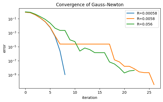
In the least perturbed case, where the minimized residual is less than 10-3, the convergence is plausibly quadratic. At the next level up, the convergence starts similarly but suddenly stagnates for a long time. In the most perturbed case, the quadratic phase is nearly gone and the overall shape looks linear.
Example 4.7.2
m = 25
V, Km = 2, 0.5
s = linspace(0.05, 6, m)
model = lambda x: V * x / (Km + x)
w = model(s) + 0.15 * cos(2 * exp(s / 16) * s)    # noise added

fig, ax = subplots()
ax.scatter(s, w, label="data")
ax.plot(s, model(s), 'k--', label="unperturbed model")
xlabel("s"), ylabel("w")
legend();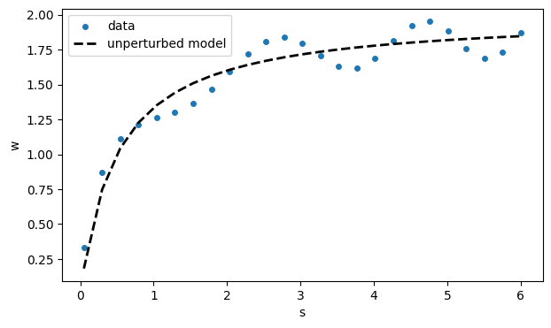
The idea is to pretend that we know nothing of the origins of this data and use nonlinear least squares to find the parameters in the theoretical model function . In (4.7.2), the variable plays the role of , and plays the role of .
Tip
Putting comma-separated values on the left of an assignment will destructure the right-hand side, drawing individual assignments from entries of a vector, for example.
def misfit(c):
    V, Km = c  # rename components for clarity
    f = V * s / (Km + s) - w
    return f
In the Jacobian the derivatives are with respect to the parameters in .
def misfitjac(x):
    V, Km = x   # rename components for clarity
    J = zeros([m, 2])
    J[:, 0] = s / (Km + s)          # d/d(V)
    J[:, 1] = -V * s / (Km + s)**2  # d/d(Km)
    return J
x1 = [1, 0.75]
x = FNC.newtonsys(misfit, misfitjac, x1)
V, Km = x[-1] # final values
print(f"estimates are V = {V:.3f}, Km = {Km:.3f}")estimates are V = 1.969, Km = 0.469
The final values are reasonably close to the values , that we used to generate the noise-free data. Graphically, the model looks close to the original data.
# since V and Km have been updated, model() is too
ax.plot(s, model(s), label="nonlinear fit")
For this particular model, we also have the option of linearizing the fit process. Rewrite the model as
for the new fitting parameters and . This corresponds to the misfit function whose entries are
for . Although this misfit is nonlinear in and , it’s linear in the unknown parameters α and β. This lets us pose and solve it as a linear least-squares problem.
from numpy.linalg import lstsq
A = array( [[1 / s[i], 1.0] for i in range(len(s))] )
z = lstsq(A, 1 / w, rcond=None)[0]
alpha, beta = z
print("alpha:", alpha, "beta:", beta)
alpha: 0.12476333709901544 beta: 0.571395910043123
The two fits are different; they do not optimize the same quantities.
linmodel = lambda x: 1 / (beta + alpha / x)
ax.plot(s, linmodel(s), label="linear fit")
ax.legend()
fig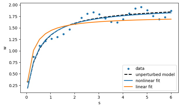
The truly nonlinear fit is clearly better in this case. It optimizes a residual for the original measured quantity rather than a transformed one we picked for algorithmic convenience.