Chapter 5 - Fundamentals of Numerical Computation

Functions¶

Hat function

hatfun.py

1
2
3
4
5
6
7
8
9
10
11
12
13
14
15
16
17
18
19
def hatfun(t, k):
    """
    hatfun(t, k)

    Returns a piecewise linear "hat" function,  where t is a vector of
    n+1 interpolation nodes and k is an integer in 0:n giving the index of the node
    where the hat function equals one.
    """
    n = len(t) - 1

    def evaluate(x):
        H = np.zeros(np.array(x).shape)
        for (j, xj) in enumerate(x):
            if (k > 0) and (t[k-1] <= xj) and (xj <= t[k]):
                H[j] = (xj - t[k-1]) / (t[k] - t[k-1])
            elif (k < n) and (t[k] <= xj) and (xj <= t[k+1]):
                H[j] = (t[k+1] - xj) / (t[k+1] - t[k])
        return H
    return evaluate

Piecewise linear interpolation

plinterp.py

1
2
3
4
5
6
7
8
9
10
11
12
13
14
15
def plinterp(t, y):
    """
    plinterp(t, y)

    Create a piecewise linear interpolating function for data values in y given at nodes
    in t.
    """
    n = len(t) - 1
    H = [hatfun(t, k) for k in range(n+1)]
    def evaluate(x):
        f = 0
        for k in range(n+1):
            f += y[k] * H[k](x)
        return f
    return evaluate

Cubic spline interpolation

spinterp.py

1
2
3
4
5
6
7
8
9
10
11
12
13
14
15
16
17
18
19
20
21
22
23
24
25
26
27
28
29
30
31
32
33
34
35
36
37
38
39
40
41
42
43
44
45
46
47
48
49
50
51
52
53
54
55
56
57
58
59
def spinterp(t, y):
    """
    spinterp(t, y)

    Create a cubic not-a-knot spline interpolating function for data values in y given at nodes in t.
    """
    n = len(t) - 1
    h = [t[i + 1] - t[i] for i in range(n)]

    # Preliminary definitions.
    Z = np.zeros([n, n])
    I = np.eye(n)
    E = I[: n - 1, :]
    J = np.eye(n) + np.diag(-np.ones(n - 1), 1)
    H = np.diag(h)

    # Left endpoint interpolation:
    AL = np.hstack([I, Z, Z, Z])
    vL = y[:-1]

    # Right endpoint interpolation:
    AR = np.hstack([I, H, H**2, H**3])
    vR = y[1:]

    # Continuity of first derivative:
    A1 = E @ np.hstack([Z, J, 2 * H, 3 * H**2])
    v1 = np.zeros(n - 1)

    # Continuity of second derivative:
    A2 = E @ np.hstack([Z, Z, J, 3 * H])
    v2 = np.zeros(n - 1)

    # Not-a-knot conditions:
    nakL = np.hstack([np.zeros(3 * n), np.hstack([1, -1, np.zeros(n - 2)])])
    nakR = np.hstack([np.zeros(3 * n), np.hstack([np.zeros(n - 2), 1, -1])])

    # Assemble and solve the full system.
    A = np.vstack([AL, AR, A1, A2, nakL, nakR])
    v = np.hstack([vL, vR, v1, v2, 0, 0])
    z = solve(A, v)

    # Break the coefficients into separate vectors.
    rows = np.arange(n)
    a = z[rows]
    b = z[n + rows]
    c = z[2 * n + rows]
    d = z[3 * n + rows]
    S = [np.poly1d([d[k], c[k], b[k], a[k]]) for k in range(n)]

    # This function evaluates the spline when called with a value for x.
    def evaluate(x):
        f = np.zeros(x.shape)
        for k in range(n):
            # Evaluate this piece's cubic at the points inside it.
            index = (x >= t[k]) & (x <= t[k + 1])
            f[index] = S[k](x[index] - t[k])
        return f

    return evaluate

Fornberg’s algorithm for finite difference weights

fdweights.py

1
2
3
4
5
6
7
8
9
10
11
12
13
14
15
16
17
18
19
20
21
22
23
24
25
26
27
28
29
30
31
32
33
def fdweights(t, m):
    """
    fdweights(t, m)

    Return weights for the mth derivative of a function at zero using values at the
    nodes in vector t.
    """
    # This is a compact implementation, not an efficient one.

    def weight(t, m, r, k):
        # Recursion for one weight.
        # Input:
        #   t   nodes (vector)
        #   m   order of derivative sought
        #   r   number of nodes to use from t (<= length(t))
        #   k   index of node whose weight is found

        if (m < 0) or (m > r):  # undefined coeffs must be zero
            c = 0
        elif (m == 0) and (r == 0):  # base case of one-point interpolation
            c = 1
        else:  # generic recursion
            if k < r:
                denom = t[r] - t[k]
                c = (t[r] * weight(t, m, r-1, k) - m * weight(t, m-1, r-1, k)) / denom
            else:
                beta = np.prod(t[r-1] - t[:r-1]) / np.prod(t[r] - t[:r])
                c = beta * (m * weight(t, m-1, r-1, r-1) - t[r-1] * weight(t, m, r-1, r-1))
        return c

    r = len(t) - 1
    w = np.zeros(t.shape)
    return np.array([ weight(t, m, r, k) for k in range(r+1) ])

Trapezoid formula for numerical integration

trapezoid.py

1
2
3
4
5
6
7
8
9
10
11
def trapezoid(f, a, b, n):
    """
    trapezoid(f, a, b, n)

    Apply the trapezoid integration formula for integrand f over interval [a,b], broken up into n equal pieces. Returns estimate, vector of nodes, and vector of integrand values at the nodes.
    """
    h = (b - a) / n
    t = np.linspace(a, b, n + 1)
    y = f(t)
    T = h * (np.sum(y[1:-1]) + 0.5 * (y[0] + y[-1]))
    return T, t, y

Adaptive integration

intadapt.py

1
2
3
4
5
6
7
8
9
10
11
12
13
14
15
16
17
18
19
20
21
22
23
24
25
26
27
28
29
30
31
32
33
34
35
36
37
38
39
40
def intadapt(f, a, b, tol):
    """
    intadapt(f, a, b, tol)

    Do adaptive integration to estimate the integral of f over [a,b] to desired
    error tolerance tol. Returns estimate and a vector of evaluation nodes used.
    """

    # Use error estimation and recursive bisection.
    def do_integral(a, fa, b, fb, m, fm, tol):
        # These are the two new nodes and their f-values.
        xl = (a + m) / 2
        fl = f(xl)
        xr = (m + b) / 2
        fr = f(xr)
        t = np.array([a, xl, m, xr, b])  # all 5 nodes at this level

        # Compute the trapezoid values iteratively.
        h = b - a
        T = np.zeros(3)
        T[0] = h * (fa + fb) / 2
        T[1] = T[0] / 2 + (h / 2) * fm
        T[2] = T[1] / 2 + (h / 4) * (fl + fr)

        S = (4 * T[1:] - T[:-1]) / 3  # Simpson values
        E = (S[1] - S[0]) / 15  # error estimate

        if abs(E) < tol * (1 + abs(S[1])):  # acceptable error?
            Q = S[1]  # yes--done
        else:
            # Error is too large--bisect and recurse.
            QL, tL = do_integral(a, fa, m, fm, xl, fl, tol)
            QR, tR = do_integral(m, fm, b, fb, xr, fr, tol)
            Q = QL + QR
            t = np.hstack([tL, tR[1:]])  # merge the nodes w/o duplicate
        return Q, t

    m = (b + a) / 2
    Q, t = do_integral(a, f(a), b, f(b), m, f(m), tol)
    return Q, t

Examples¶

5.1 The interpolation problem¶

Example 5.1.1

Here are some points that we could consider to be observations of an unknown function on $[-1,1]$ .

n = 5
t = linspace(-1, 1, n + 1)
y = t**2 + t + 0.05 * sin(20 * t)
fig, ax = subplots()
plot(t, y, "o", label="data")
xlabel("$x$"),  ylabel("$y$");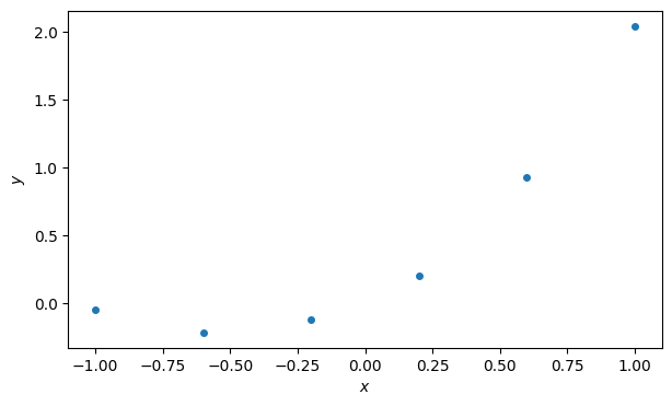

The polynomial interpolant, as computed using fit, looks very sensible. It’s the kind of function you’d take home to meet your parents.

p = poly1d(polyfit(t, y, n))  # interpolating polynomial
tt = linspace(-1, 1, 400)
ax.plot(tt, p(tt), label="interpolant")
ax.legend()
fig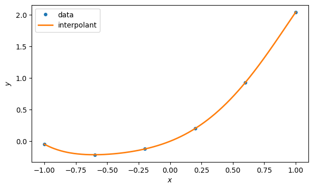

But now consider a different set of points generated in almost exactly the same way.

n = 18
t = linspace(-1, 1, n + 1)
y = t**2 + t + 0.05 * sin(20 * t)
fig, ax = subplots()
plot(t, y, "o", label="data")
xlabel("$x$"),  ylabel("$y$");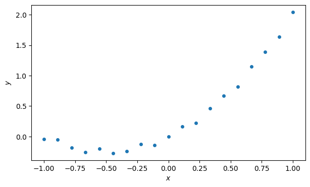

The points themselves are unremarkable. But take a look at what happens to the polynomial interpolant.

p = poly1d(polyfit(t, y, n))
ax.plot(tt, p(tt), label="interpolant")
ax.legend()
fig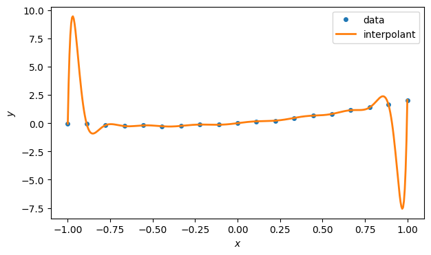

Surely there must be functions that are more intuitively representative of those points!

Example 5.1.3

Let us recall the data from Demo 5.1.1.

clf
n = 12
t = linspace(-1, 1, n + 1)
y = t**2 + t + 0.5 * sin(20 * t)
fig, ax = subplots()
scatter(t, y, label="data")
xlabel("$x$"),  ylabel("$y$");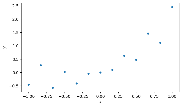

Here is an interpolant that is linear between each consecutive pair of nodes, using plinterp from Piecewise linear interpolation.

from scipy.interpolate import interp1d
tt = linspace(-1, 1, 400)
p = interp1d(t, y, kind="linear")
ax.plot(tt, p(tt), label="piecewise linear")
ax.legend()
fig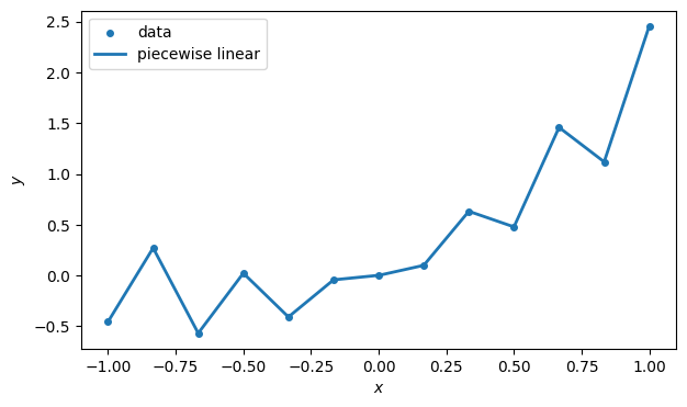

We may prefer a smoother interpolant that is piecewise cubic:

scatter(t, y, label="data")
p = interp1d(t, y, kind="cubic")
tt = linspace(-1, 1, 400)
plot(tt, p(tt), label="cubic spline")
xlabel("$x$"),  ylabel("$y$")
legend();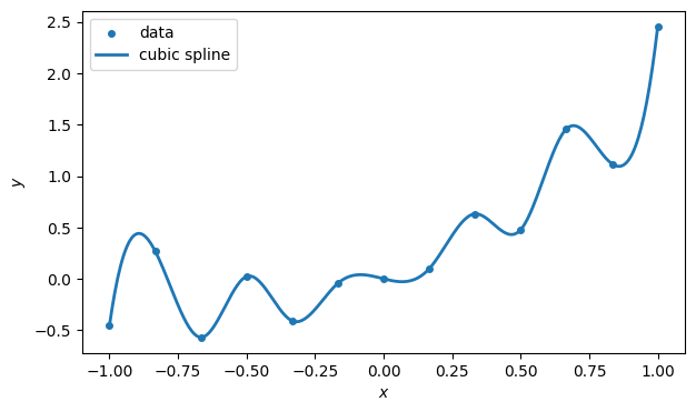

Example 5.1.4

In Demo 5.1.1 and Demo 5.1.3 we saw a big difference between polynomial interpolation and piecewise polynomial interpolation of some arbitrarily chosen data. The same effects can be seen clearly in the cardinal functions, which are closely tied to the condition numbers.

clf
n = 18
t = linspace(-1, 1, n + 1)
y = zeros(n + 1)
y[9] = 1.0
p = interp1d(t, y, kind="cubic")

scatter(t, y, label="data")
tt = linspace(-1, 1, 400)
plot(tt, p(tt), label="cardinal function")
title("Cubic spline cardinal function")
legend();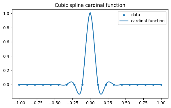

The piecewise cubic cardinal function is nowhere greater than one in absolute value. This happens to be true for all the cardinal functions, ensuring a good condition number for any interpolation with these functions. But the story for global polynomials is very different.

p = poly1d(polyfit(t, y, n))
scatter(t, y, label="data")
plot(tt, p(tt), label="cardinal function")
xlabel("$x$")
ylabel("$y$")
title("Polynomial cardinal function")
legend();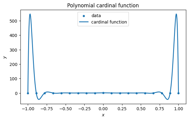

From the figure we can see that the condition number for polynomial interpolation on these nodes is at least 500.

5.2 Piecewise linear interpolation¶

Example 5.2.1

Let’s define a set of four nodes (i.e., $n=3$ in our formulas).

t = array([0, 0.075, 0.25, 0.55, 0.7, 1])

We plot the hat functions $H_0,\ldots,H_3$ .

x = linspace(0, 1, 300)
for k in range(6):
    plot(x, FNC.hatfun(t, k)(x))
xlabel("$x$"),  ylabel("$H_k(x)$")
title("Hat functions");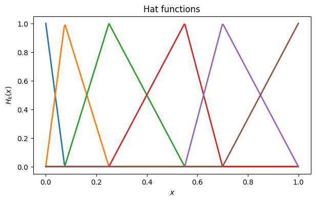

Example 5.2.2

We generate a piecewise linear interpolant of $f(x)=e^{\sin 7x}$ .

f = lambda x: exp(sin(7 * x))
x = linspace(0, 1, 400)
fig, ax = subplots()
plot(x, f(x), label="function")
xlabel("$x$")
ylabel("$f(x)$");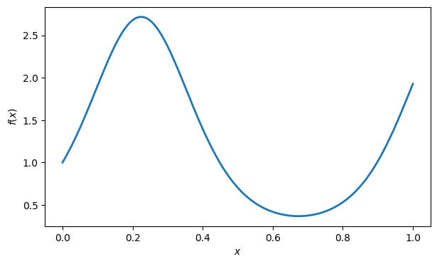

First we sample the function to create the data.

t = array([0, 0.075, 0.25, 0.55, 0.7, 1])  # nodes
y = f(t)  # function values

ax.plot(t, y, "o", label="nodes")
ax.legend()
fig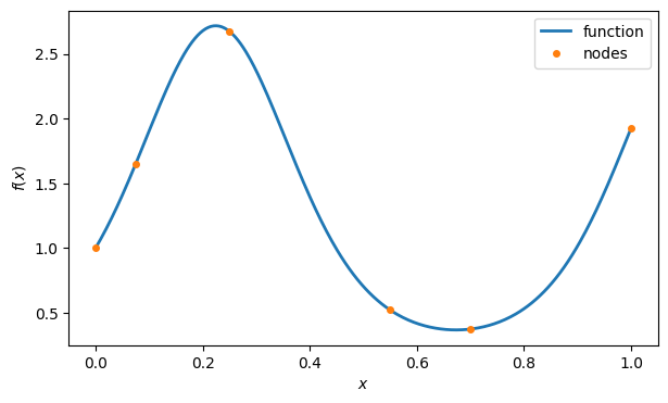

Now we create a callable function that will evaluate the piecewise linear interpolant at any $x$ , and then plot it.

p = FNC.plinterp(t, y)
ax.plot(x, p(x), label="interpolant")
ax.legend()
fig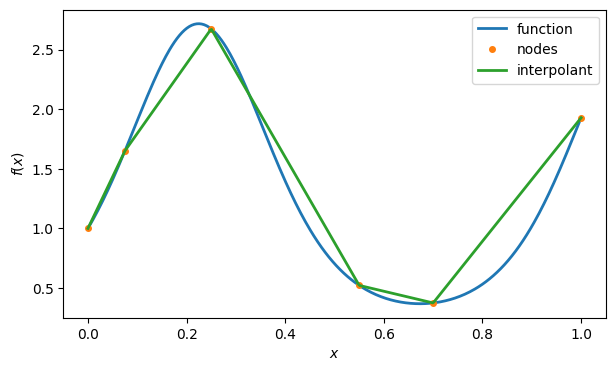

Example 5.2.3

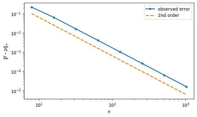
We measure the convergence rate for piecewise linear interpolation of $e^{\sin 7x}$ over $x \in [0,1]$ .

f = lambda x: exp(sin(7 * x))
x = linspace(0, 1, 10000)  # sample the difference at many points
N = 2 ** arange(3, 11)
err = zeros(N.size)
for i, n in enumerate(N):
    t = linspace(0, 1, n + 1)  # interpolation nodes
    p = FNC.plinterp(t, f(t))
    err[i] = max(abs(f(x) - p(x)))
print(err)

[2.16029984e-01 6.38173511e-02 1.60381329e-02 4.05882168e-03
 1.01556687e-03 2.54022468e-04 6.35007579e-05 1.58778800e-05]

As predicted, a factor of 10 in $n$ produces a factor of 100 in the error. In a convergence plot, it is traditional to have $h$ decrease from left to right, so we expect a straight line of slope -2 on a log-log plot.

order2 = 0.1 * (N / N[0]) ** (-2)
loglog(N, err, "-o", label="observed error")
loglog(N, order2, "--", label="2nd order")
xlabel("$n$")
ylabel("$\|f-p\|_\infty$")
legend();

<>:5: SyntaxWarning: invalid escape sequence '\|'
<>:5: SyntaxWarning: invalid escape sequence '\|'
/var/folders/gc/0752xrm56pnf0r0dsrn5370c0000gr/T/ipykernel_93662/3346807096.py:5: SyntaxWarning: invalid escape sequence '\|'
  ylabel("$\|f-p\|_\infty$")

5.3 Cubic splines¶

Example 5.3.1

For illustration, here is a spline interpolant using just a few nodes.

f = lambda x: exp(sin(7 * x))

x = linspace(0, 1, 500)
fig, ax = subplots()
ax.plot(x, f(x), label="function")

t = array([0, 0.075, 0.25, 0.55, 0.7, 1])  # nodes
y = f(t)  # values at nodes

xlabel("$x$")
ylabel("$y$")
ax.scatter(t, y, label="nodes")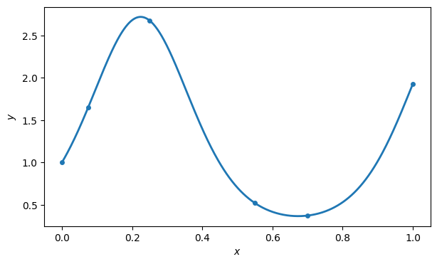

S = FNC.spinterp(t, y)
ax.plot(x, S(x), label="spline")
ax.legend()
fig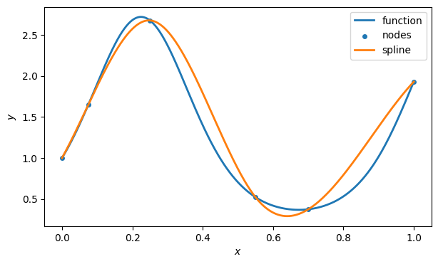

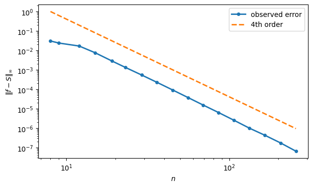
Now we look at the convergence rate as the number of nodes increases.

N = floor(2 ** linspace(3, 8, 17)).astype(int)
err = zeros(N.size)
for i, n in enumerate(N):
    t = linspace(0, 1, n + 1)  # interpolation nodes
    p = FNC.spinterp(t, f(t))
    err[i] = max(abs(f(x) - p(x)))
print(err)

[3.05633432e-02 2.39601586e-02 1.68054365e-02 7.64098319e-03
 2.89472870e-03 1.34574135e-03 5.43142890e-04 2.28104055e-04
 9.17629364e-05 3.71552636e-05 1.56015311e-05 6.34890672e-06
 2.53866817e-06 9.98323636e-07 4.35498457e-07 1.75251504e-07
 6.59321329e-08]

Since we expect convergence that is $O(h^4)=O(n^{-4})$ , we use a log-log graph of error and expect a straight line of slope -4.

order4 = (N / N[0]) ** (-4)
loglog(N, err, "-o", label="observed error")
loglog(N, order4, "--", label="4th order")
xlabel("$n$")
ylabel("$\|f-S\|_\infty$")
legend();

<>:5: SyntaxWarning: invalid escape sequence '\|'
<>:5: SyntaxWarning: invalid escape sequence '\|'
/var/folders/gc/0752xrm56pnf0r0dsrn5370c0000gr/T/ipykernel_93662/3396180238.py:5: SyntaxWarning: invalid escape sequence '\|'
  ylabel("$\|f-S\|_\infty$")

5.4 Finite differences¶

Example 5.4.3

If $f(x)=e^{\,\sin(x)}$ , then $f'(0)=1$ .

f = lambda x: exp(sin(x))

Here are the first two centered differences from Table 5.4.1.

h = 0.05
CD2 = (-f(-h) + f(h)) / (2*h)
CD4 = (f(-2*h) - 8*f(-h) + 8*f(h) - f(2*h)) / (12*h)
print(f"CD2 is {CD2:.9f} and CD4 is {CD4:.9f}")

CD2 is 0.999999584 and CD4 is 1.000001663

Here are the first two forward differences from Table 5.4.2.

FD1 = (-f(0) + f(h)) / h
FD2 = (-3*f(0) + 4*f(h) - f(2*h)) / (2*h)
print(f"FD1 is {FD1:.9f} and FD2 is {FD2:.9f}")

FD1 is 1.024983957 and FD2 is 1.000099611

Finally, here are the backward differences that come from reverse-negating the forward differences.

BD1 = (-f(-h) + f(0)) / h
BD2 = (f(-2*h) - 4*f(-h) + 3*f(0)) / (2*h)
print(f"BD1 is {BD1:.9f} and BD2 is {BD2:.9f}")

BD1 is 0.975015210 and BD2 is 0.999912034

Example 5.4.4

If $f(x)=e^{\,\sin(x)}$ , then $f''(0)=1$ .

f = lambda x: exp(sin(x))

Here is a centered estimate given by (5.4.12).

h = 0.05
CD2 = (f(-h) - 2*f(0) + f(h)) / h**2
print(f"CD2 is {CD2:.9f}")

CD2 is 0.999374948

For the same $h$ , here are forward estimates given by (5.4.13) and (5.4.14).

FD1 = (f(0) - 2*f(h) + f(2*h)) / h**2
FD2 = (2*f(0) - 5*f(h) + 4*f(2*h) - f(3*h)) / h**2
print(f"FD1 is {FD1:.9f} and FD2 is {FD2:.9f}")

FD1 is 0.995373844 and FD2 is 1.007881148

Finally, here are the backward estimates that come from reversing (5.4.13) and (5.4.14).

BD1 = (f(-2*h) - 2*f(-h) + f(0)) / h**2
BD2 = (-f(-3*h) + 4*f(-2*h) - 5*f(-h) + 2*f(0)) / h**2
print(f"BD1 is {BD1:.9f} and BD2 is {BD2:.9f}")

BD1 is 0.995872969 and BD2 is 1.005892819

Example 5.4.5

We will estimate the derivative of $\cos(x^2)$ at $x=0.5$ using five nodes.

t = array([0.35, 0.5, 0.57, 0.6, 0.75])   # nodes
f = lambda x: cos(x**2)
dfdx = lambda x: -2 * x * sin(x**2)
exact_value = dfdx(0.5)

We have to shift the nodes so that the point of estimation for the derivative is at $x=0$ . (To subtract a scalar from a vector, we must use the .- operator.)

w = FNC.fdweights(t - 0.5, 1)

The finite-difference formula is a dot product (i.e., inner product) between the vector of weights and the vector of function values at the nodes.

fd_value = dot(w, f(t))

We can reproduce the weights in the finite-difference tables by using equally spaced nodes with $h=1$ . For example, here is a one-sided formula at four nodes.

print(FNC.fdweights(linspace(0, 3, 4), 1))

[-1.83333333  3.         -1.5         0.33333333]

5.5 Convergence of finite differences¶

Example 5.5.3

Let’s observe the convergence of the formulas in Example 5.5.1 and Example 5.5.2, applied to the function $\sin(e^{x+1})$ at $x=0$ .

f = lambda x: sin(exp(x + 1))
exact_value = exp(1) * cos(exp(1))

We’ll compute the formulas in parallel for a sequence of $h$ values.

h_ = array([5 / 10**(n+1) for n in range(6)])
FD = zeros((len(h_), 2))
for (i, h) in enumerate(h_):
    FD[i, 0] = (f(h) - f(0)) / h 
    FD[i, 1] = (f(h) - f(-h)) / (2*h)
results = PrettyTable()
results.add_column("h", h_)
results.add_column("FD1", FD[:, 0])
results.add_column("FD2", FD[:, 1])
print(results)

+--------+---------------------+---------------------+
|   h    |         FD1         |         FD2         |
+--------+---------------------+---------------------+
|  0.5   |  -2.768575766550465 | -1.9704719803862911 |
|  0.05  | -2.6127952856136947 |  -2.475520256824717 |
| 0.005  | -2.4921052189334048 | -2.4783216951179465 |
| 0.0005 | -2.4797278609705042 | -2.4783494526022243 |
| 5e-05  | -2.4784875710526233 |  -2.478349730152263 |
| 5e-06  |  -2.478363517077753 |  -2.478349732970564 |
+--------+---------------------+---------------------+

All that’s easy to see from this table is that FD2 appears to converge to the same result as FD1, but more rapidly. A table of errors is more informative.

errors = FD - exact_value
results = PrettyTable()
results.add_column("h", h_)
results.add_column("error in FD1", errors[:, 0])
results.add_column("error in FD2", errors[:, 1])
print(results)

+--------+-------------------------+------------------------+
|   h    |       error in FD1      |      error in FD2      |
+--------+-------------------------+------------------------+
|  0.5   |   -0.29022603359523025  |   0.5078777525689437   |
|  0.05  |   -0.1344455526584598   | 0.0028294761305178717  |
| 0.005  |   -0.01375548597816989  | 2.8037837288330536e-05 |
| 0.0005 |  -0.0013781280152693753 | 2.8035301058437767e-07 |
| 5e-05  |  -0.0001378380973884319 | 2.8029720766653554e-09 |
| 5e-06  | -1.3784122518067932e-05 | -1.532907134560446e-11 |
+--------+-------------------------+------------------------+

In each row, $h$ is decreased by a factor of 10, so that the error is reduced by a factor of 10 in the first-order method and 100 in the second-order method.

A graphical comparison can be useful as well. On a log-log scale, the error should (as $h\to 0$ ) be a straight line whose slope is the order of accuracy. However, it’s conventional in convergence plots to show $h$ decreasing from left to right, which negates the slopes.

plot(h_, abs(errors), "o-", label=["FD1", "FD2"])
gca().invert_xaxis()
# Add lines for perfect 1st and 2nd order.
loglog(h_, h_, "--", label="$O(h)$")
loglog(h_, h_**2, "--", label="$O(h^2)$")
xlabel("$h$")
ylabel("error")
legend();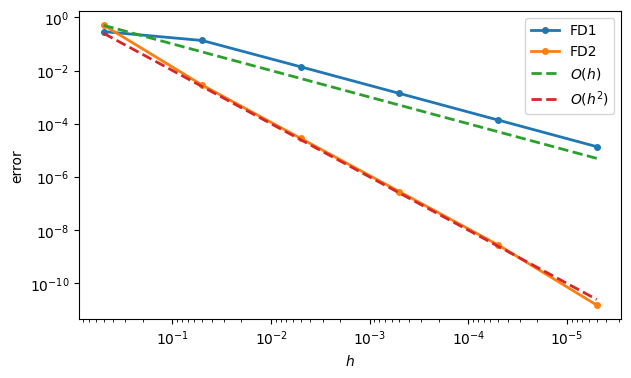

Example 5.5.4

Let $f(x)=e^{-1.3x}$ . We apply finite-difference formulas of first, second, and fourth order to estimate $f'(0)=-1.3$ .

f = lambda x: exp(-1.3 * x)
exact = -1.3

h_ = array([1 / 10**(n+1) for n in range(12)])
FD = zeros((len(h_), 3))
for (i, h) in enumerate(h_):
    nodes = h * linspace(-2, 2, 5)
    vals = f(nodes)
    FD[i, 0] = dot(array([0, 0, -1, 1, 0]) / h, vals)
    FD[i, 1] = dot(array([0, -1/2, 0, 1/2, 0]) / h, vals)
    FD[i, 2] = dot(array([1/12, -2/3, 0, 2/3, -1/12]) / h, vals)

results = PrettyTable()
results.add_column("h", h_)
results.add_column("FD1", FD[:, 0])
results.add_column("FD2", FD[:, 1])
results.add_column("FD4", FD[:, 2])
print(results)

+--------+---------------------+---------------------+---------------------+
|   h    |         FD1         |         FD2         |         FD4         |
+--------+---------------------+---------------------+---------------------+
|  0.1   | -1.2190456907943865 | -1.3036647620203026 |  -1.299987598641898 |
|  0.01  | -1.2915864979712381 | -1.3000366169760815 | -1.2999999987623418 |
| 0.001  | -1.2991553660477848 | -1.3000003661667074 | -1.2999999999999687 |
| 0.0001 | -1.2999155036613956 |  -1.300000003662075 | -1.3000000000002956 |
| 1e-05  | -1.2999915500404313 | -1.3000000000396366 | -1.3000000000138243 |
| 1e-06  |  -1.299999154987745 | -1.2999999999900496 | -1.3000000000320142 |
| 1e-07  | -1.2999999150633812 | -1.3000000000289944 |  -1.300000001094304 |
| 1e-08  | -1.2999999970197678 | -1.3000000042305544 | -1.3000000128522515 |
| 1e-09  | -1.2999999523162842 | -1.3000000340328768 | -1.3000001162290573 |
| 1e-10  | -1.2999992370605469 | -1.2999996723115146 | -1.3000001907348633 |
| 1e-11  | -1.3000030517578125 | -1.3000038001061966 | -1.3000049591064453 |
| 1e-12  |   -1.2999267578125  |  -1.300004483829298 | -1.3000030517578125 |
+--------+---------------------+---------------------+---------------------+

They all seem to be converging to -1.3. The convergence plot reveals some interesting structure to the errors, though.

loglog(h_, abs(FD[:, 0] + 1.3), "-o", label="FD1")
loglog(h_, abs(FD[:, 1] + 1.3), "-o", label="FD2")
loglog(h_, abs(FD[:, 2] + 1.3), "-o", label="FD4")
gca().invert_xaxis()
plot(h_, 0.1 * 2 ** (-52) / h_, "--", color="k", label="$O(h^{-1})$")
xlabel("$h$")
ylabel("total error")
title("FD error with roundoff")
legend();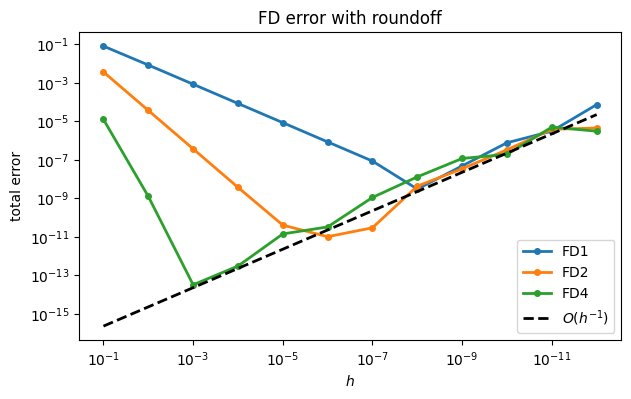

Again the graph is made so that $h$ decreases from left to right. The errors are dominated at first by truncation error, which decreases most rapidly for the fourth-order formula. However, increasing roundoff error eventually equals and then dominates the truncation error as $h$ continues to decrease. As the order of accuracy increases, the crossover point moves to the left (greater efficiency) and down (greater accuracy).

5.6 Numerical integration¶

Example 5.6.1

The antiderivative of $e^x$ is, of course, itself. That makes evaluation of $\int_0^1 e^x\,dx$ by the Fundamental Theorem trivial.

exact = exp(1) - 1

The module scipy.integrate has multiple functions that estimate the value of an integral numerically without finding the antiderivative first. As you can see here, it’s often just as accurate.

from scipy.integrate import quad
Q, errest = quad(exp, 0, 1, epsabs=1e-13, epsrel=1e-13)
print(Q)

1.7182818284590453

The numerical approach is also far more robust. For example, $e^{\,\sin x}$ has no useful antiderivative. But numerically, it’s no more difficult.

Q, errest = quad(lambda x: exp(sin(x)), 0, 1, epsabs=1e-13, epsrel=1e-13)
print(Q)

1.6318696084180513

When you look at the graphs of these functions, what’s remarkable is that one of these areas is basic calculus while the other is almost impenetrable analytically. From a numerical standpoint, they are practically the same problem.

x = linspace(0, 1, 300)
subplot(1, 2, 1)
plot(x, exp(x))
ylim([0, 2.7]), title("exp(x)")
subplot(1, 2, 2)
plot(x, exp(sin(x)))
ylim([0, 2.7]), title("exp(sin(x))");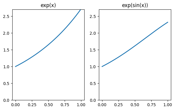

Example 5.6.2

We will approximate the integral of the function $f(x)=e^{\sin 7x}$ over the interval $[0,2]$ .

f = lambda x: exp(sin(7 * x))
a, b = 0, 2

In lieu of the exact value, we will use the quad function to find an accurate result.

from scipy.integrate import quad
I, errest = quad(f, a, b, epsabs=1e-13, epsrel=1e-13)
print(f"Integral = {I:.14f}")

Integral = 2.66321978276154

Here is the trapezoid result at $n=40$ , and its error.

T, t, y = FNC.trapezoid(f, a, b, 40)
print(f"Trapezoid estimate is {T:.14f} with error {I - T:.2e}")

Trapezoid estimate is 2.66230293560229 with error 9.17e-04

In order to check the order of accuracy, we increase $n$ by orders of magnitude and observe how the error decreases.

n_ = 40 * 2 ** arange(6)
err = zeros(size(n_))
print("     n     error")
for k, n in enumerate(n_):
    T, t, y = FNC.trapezoid(f, a, b, n)
    err[k] = I - T
    print(f"{n:6d}   {err[k]:8.3e} ")

     n     error
    40   9.168e-04 
    80   2.301e-04 
   160   5.757e-05 
   320   1.440e-05 
   640   3.599e-06 
  1280   8.998e-07

Each increase by a factor of 10 in $n$ cuts the error by a factor of about 100, which is consistent with second-order convergence. Another check is that a log-log graph should give a line of slope -2 as $n\to\infty$ .

loglog(n_, abs(err), "-o", label="results")
loglog(n_, 3e-3 * (n_ / n_[0]) ** (-2), "--", label="2nd order")
gca().invert_xaxis()
xlabel("$n$")
ylabel("error")
legend()
title("Convergence of trapezoidal integration");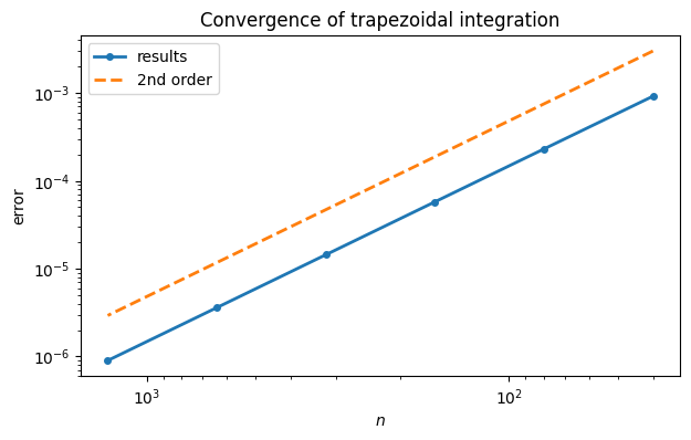

Example 5.6.3

We estimate $\displaystyle\int_0^2 x^2 e^{-2x}\, dx$ using extrapolation. First we use quadgk to get an accurate value.

from scipy.integrate import quad
f = lambda x: x**2 * exp(-2 * x)
a = 0
b = 2
I, errest = quad(f, a, b, epsabs=1e-13, epsrel=1e-13)
print(f"Integral = {I:.14f}")

Integral = 0.19047417361161

We start with the trapezoid formula on $n=N$ nodes.

N = 20    # the coarsest formula
n = N
h = (b - a) / n
t = h * arange(n + 1)
y = f(t)

We can now apply weights to get the estimate $T_f(N)$ .

T = zeros(3)
T[0] = h * (sum(y[1:-1]) + y[0] / 2 + y[-1] / 2)
print(f"error (2nd order): {I - T[0]:.2e}")

error (2nd order): 6.27e-05

Now we double to $n=2N$ , but we only need to evaluate $f$ at every other interior node and apply (5.6.18).

n = 2 * n
h = h / 2
t = h * arange(n + 1)
T[1] = T[0] / 2 + h * sum(f(t[1:-1:2]))
print("error (2nd order):", I - T[:2])

error (2nd order): [6.27236723e-05 1.53677521e-05]

As expected for a second-order estimate, the error went down by a factor of about 4. We can repeat the same code to double $n$ again.

n = 2 * n
h = h / 2
t = h * arange(n + 1)
T[2] = T[1] / 2 + h * sum(f(t[1:-1:2]))
print("error (2nd order):", I - T[:3])

error (2nd order): [6.27236723e-05 1.53677521e-05 3.82230697e-06]

Let us now do the first level of extrapolation to get results from Simpson’s formula. We combine the elements T[i] and T[i+1] the same way for $i=1$ and $i=2$ .

S = array([(4 * T[i + 1] - T[i]) / 3 for i in range(2)])
print("error (4th order):", I - S)

error (4th order): [-4.17554646e-07 -2.61747412e-08]

With the two Simpson values $S_f(N)$ and $S_f(2N)$ in hand, we can do one more level of extrapolation to get a sixth-order accurate result.

R = (16 * S[1] - S[0]) / 15
print("error (6th order):", I - R)

error (6th order): -8.274758656057202e-11

We can make a triangular table of the errors:

err = nan * ones((3, 3))
err[0, :] = I - T
err[1, 1:] = I - S
err[2, 2] = I - R
results = PrettyTable(["2nd order", "4th order", "6th order"])
results.add_rows(err.T)
print(results)

+------------------------+-------------------------+------------------------+
|       2nd order        |        4th order        |       6th order        |
+------------------------+-------------------------+------------------------+
| 6.272367234608223e-05  |           nan           |          nan           |
| 1.5367752102174448e-05 | -4.1755464580406354e-07 |          nan           |
| 3.822306969658573e-06  | -2.6174741207807273e-08 | -8.274758656057202e-11 |
+------------------------+-------------------------+------------------------+

If we consider the computational time to be dominated by evaluations of $f$ , then we have obtained a result with about twice as many accurate digits as the best trapezoid result, at virtually no extra cost.

5.7 Adaptive integration¶

Example 5.7.1

This function gets increasingly oscillatory as $x$ increases.

f = lambda x: (x + 1) ** 2 * cos((2 * x + 1) / (x - 4.3))
x = linspace(0, 4, 600)
plot(x, f(x))
xlabel("$x$")
ylabel("$f(x)$");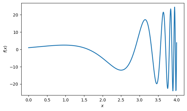

Accordingly, the trapezoid rule is more accurate on the left half of this interval than on the right half.

n_ = 50 * 2 ** arange(4)
Tleft = zeros(4)
Tright = zeros(4)
for i, n in enumerate(n_):
    Tleft[i] = FNC.trapezoid(f, 0, 2, n)[0]
    Tright[i] = FNC.trapezoid(f, 2, 4, n)[0]
print("left half:", Tleft)
print("right half:", Tright)

left half: [2.00419122 2.00605957 2.00652661 2.00664337]
right half: [-4.32798637 -4.73621129 -4.80966839 -4.82666144]

from scipy.integrate import quad
left_val, err = quad(f, 0, 2, epsabs=1e-13, epsrel=1e-13)
right_val, err = quad(f, 2, 4, epsabs=1e-13, epsrel=1e-13)

print("    n     left error   right error")
for k in range(n_.size):
    print(f"  {n_[k]:4}    {Tleft[k]-left_val:8.3e}    {Tright[k]-right_val:8.3e}")

    n     left error   right error
    50    -2.491e-03    5.042e-01
   100    -6.227e-04    9.600e-02
   200    -1.557e-04    2.255e-02
   400    -3.892e-05    5.554e-03

Both the picture and the numerical results suggest that more nodes should be used on the right half of the interval than on the left half.

Example 5.7.2

We’ll integrate the function from Demo 5.7.1.

from scipy.integrate import quad
f = lambda x: (x + 1) ** 2 * cos((2 * x + 1) / (x - 4.3))
I, errest = quad(f, 0, 4, epsabs=1e-12, epsrel=1e-12)
print("integral:", I)    # 'exact' value

integral: -2.8255333734374504

We perform the integration and show the nodes selected underneath the curve.

Q, t = FNC.intadapt(f, 0, 4, 0.001)
print("number of nodes:", t.size)

x = linspace(0, 4, 600)
plot(x, f(x), "k")
stem(t, f(t))
xlabel("$x$"); ylabel("$f(x)$");

number of nodes: 69

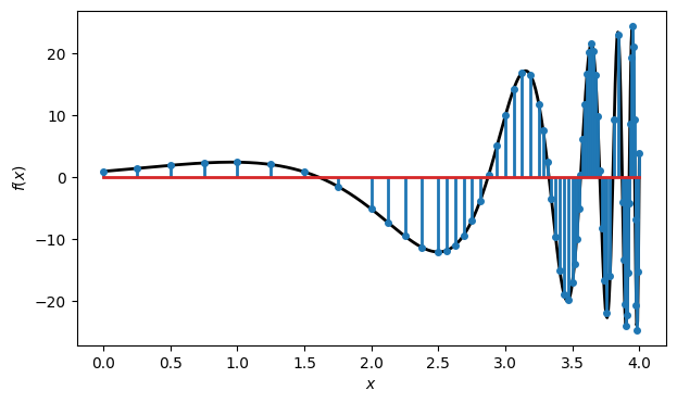
The error turns out to be a bit more than we requested. It’s only an estimate, not a guarantee.

print("error:", I - Q)

error: -0.02200281303763152

Let’s see how the number of integrand evaluations and the error vary with the requested tolerance.

tol_ = 10.0 ** arange(-4, -12, -1)
err_ = zeros(tol_.size)
num_ = zeros(tol_.size, dtype=int)
print("    tol         error     # f-evals")
for i, tol in enumerate(tol_):
    Q, t = FNC.intadapt(f, 0, 4, tol)
    err_[i] = I - Q
    num_[i] = t.size
    print(f"  {tol:6.1e}    {err_[i]:10.3e}    {num_[i]:6d}")

    tol         error     # f-evals
  1.0e-04    -4.195e-04       113
  1.0e-05     4.790e-05       181
  1.0e-06     6.314e-06       297
  1.0e-07    -6.639e-07       489
  1.0e-08     7.181e-08       757
  1.0e-09     1.265e-08      1193
  1.0e-10    -8.441e-10      2009
  1.0e-11     2.612e-11      3157

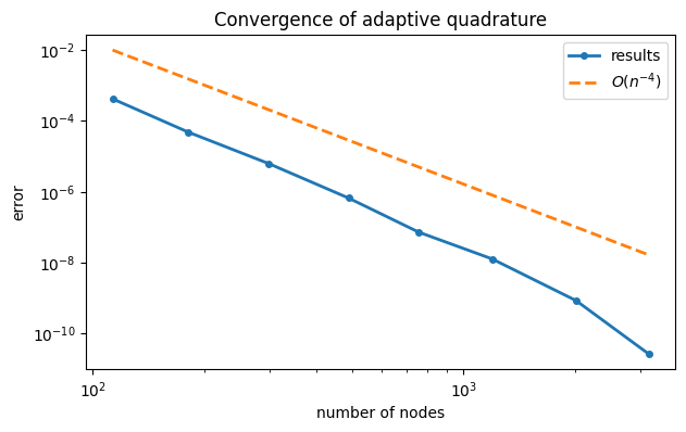
As you can see, even though the errors are not smaller than the estimates, the two columns decrease in tandem. If we consider now the convergence not in $h$ , which is poorly defined now, but in the number of nodes actually chosen, we come close to the fourth-order accuracy of the underlying Simpson scheme.

loglog(num_, abs(err_), "-o", label="results")
order4 = 0.01 * (num_ / num_[0]) ** (-4)
loglog(num_, order4, "--", label="$O(n^{-4})$")
xlabel("number of nodes"), ylabel("error")
legend()
title("Convergence of adaptive quadrature");