Chapter 10 - Fundamentals of Numerical Computation

Functions¶

Shooting method for a two-point boundary-value problem

shoot.m

1
2
3
4
5
6
7
8
9
10
11
12
13
14
15
16
17
18
19
20
21
22
23
24
25
26
27
28
29
30
31
32
33
34
35
36
37
38
39
40
41
function [x, u, du_dx] = shoot(phi, a, b, ga, gb, init, tol)
%SHOOT   Shooting method for a two-point boundary-value problem.
% Input:
%   phi      defines u'' = phi(x, u, u') (function)
%   a, b     endpoints of the domain (scalars)
%   ga       residual boundary function of u(a), u'(a) 
%   gb       residual boundary function of u(b), u'(b) 
%   init     initial guess for u(a) and u'(a) (column vector)
%   tol      error tolerance (scalar)
% Output:
%   x        nodes in x (length n+1)
%   u        values of u(x)  (length n+1)
%   du_dx    values of u'(x) (length n+1)

% To be solved by the IVP solver
function f = shootivp(x, y)
  f = [ y(2); phi(x, y(1), y(2)) ];
end

ivp = ode(ODEFcn=@shootivp);
ivp.InitialTime = a;
ivp.AbsoluteTolerance = tol / 10;
ivp.RelativeTolerance = tol / 10;

% To be solved by levenberg
function residual = objective(s)
  ivp.InitialValue = s;
  sol = solve(ivp, a, b);
  x = sol.Time;  y = sol.Solution;
  residual = [ga(y(1, 1), y(2, 1)); gb(y(1, end), y(2, end))];
end

y = [];    % shared variable
s = levenberg(@objective, init, tol);

% Don't need to solve the IVP again. It was done within the
% objective function already.
u = y(1, :);            % solution     
du_dx = y(2, :);         % derivative

end

Second-order differentiation matrices

diffmat2.m

1
2
3
4
5
6
7
8
9
10
11
12
13
14
15
16
17
18
19
20
21
22
23
24
25
26
27
28
29
30
31
32
function [x,Dx,Dxx] = diffmat2(n,xspan)
%DIFFMAT2   Second-order accurate differentiation matrices.
% Input:
%   n       number of subintervals (one less than the number of nodes)
%   xspan   interval endpoints
% Output:
%   x       equispaced nodes
%   Dx      matrix for first derivative 
%   Dxx     matrix for second derivative 

a = xspan(1);  b = xspan(2);
h = (b-a)/n;
x = a + h*(0:n)';   % nodes

% Define most of Dx by its diagonals.
dp = 0.5*ones(n,1)/h;       % superdiagonal
dm = -0.5*ones(n,1)/h;      % subdiagonal
Dx = diag(dm,-1) + diag(dp,1);

% Fix first and last rows.
Dx(1,1:3) = [-1.5,2,-0.5]/h;
Dx(n+1,n-1:n+1) = [0.5,-2,1.5]/h;

% Define most of Dxx by its diagonals.
d0 =  -2*ones(n+1,1)/h^2;   % main diagonal
dp =  ones(n,1)/h^2;        % superdiagonal and subdiagonal
Dxx = diag(dp,-1) + diag(d0) + diag(dp,1);

% Fix first and last rows.
Dxx(1,1:4) = [2,-5,4,-1]/h^2;
Dxx(n+1,n-2:n+1) = [-1,4,-5,2]/h^2;

Chebyshev differentiation matrices

diffcheb.m

1
2
3
4
5
6
7
8
9
10
11
12
13
14
15
16
17
18
19
20
21
22
23
24
25
26
27
28
29
30
31
32
33
function [x,Dx,Dxx] = diffcheb(n,xspan)
%DIFFCHEB   Chebyshev differentiation matrices.
% Input:
%   n      number of subintervals (integer)
%   xspan  interval endpoints (vector)
% Output:
%   x      Chebyshev nodes in domain (length n+1)
%   Dx     matrix for first derivative (n+1 by n+1)
%   Dxx    matrix for second derivative (n+1 by n+1)

x = -cos( (0:n)'*pi/n );    % nodes in [-1,1]
Dx = zeros(n+1);
c = [2; ones(n-1,1); 2];    % endpoint factors
i = (0:n)';                 % row indices

% Off-diagonal entries
for j = 0:n
  num = c(i+1).*(-1).^(i+j);
  den = c(j+1)*(x-x(j+1));
  Dx(:,j+1) = num./den;
end

% Diagonal entries
Dx(isinf(Dx)) = 0;          % fix divisions by zero on diagonal
Dx = Dx - diag(sum(Dx,2));  % "negative sum trick" 
  
% Transplant to [a,b]
a = xspan(1);  b = xspan(2);
x = a + (b-a)*(x+1)/2;
Dx = 2*Dx/(b-a);

% Second derivative
Dxx = Dx^2;

Solution of a linear boundary-value problem

bvplin.m

1
2
3
4
5
6
7
8
9
10
11
12
13
14
15
16
17
18
19
20
21
22
23
24
25
26
27
function [x, u] = bvplin(p, q, r, a, b, ua, ub,n)
% BVPLIN   Solve a linear boundary-value problem.
% Input:
%   p, q, r  u'' + pu' + qu = r (functions)
%   a, b     endpoints of the domain (scalars)
%   ua       value of u(a)
%   ub       value of u(b)
%   n        number of subintervals (integer)
% Output:
%   x       collocation nodes (vector, length n+1)
%   u       solution at nodes (vector, length n+1)

[x, Dx, Dxx] = diffmat2(n, [a, b]);

P = diag(p(x));
Q = diag(q(x));
L = Dxx + P * Dx + Q;    % ODE expressed at the nodes
r = r(x);    

% Replace first and last rows using boundary conditions. 
I = speye(n+1); 
A = [ I(:, 1)'; L(2:n, :); I(:, n+1)' ];

f = [ ua; r(2:n); ub ];

% Solve the system.
u = A \ f;

Solution of a nonlinear boundary-value problem

bvp.m

1
2
3
4
5
6
7
8
9
10
11
12
13
14
15
16
17
18
19
20
21
22
23
24
25
26
27
28
29
30
31
32
33
34
  function [x,u] = bvp(phi, a, b, ga, gb, init)
%BVP      Solve a boundary-value problem by finite differences
%         with either Dirichlet or Neumann BCs.
% Input:
%   phi      defines u'' = phi(x,u,u') (function)
%   a, b     endpoints of the domain (scalars)
%   ga       residual boundary function of u(a), u'(a) 
%   gb       residual boundary function of u(b), u'(b) 
%   init     initial guess for the solution (length n+1 vector)
% Output:
%   x        nodes in x (vector, length n+1)
%   u        values of u(x)  (vector, length n+1)
%   res      function for computing the residual

n = length(init) - 1;
[x, Dx, Dxx] = diffmat2(n, [a, b]);
h = x(2) - x(1);

u = levenberg(@residual, init);
u = u(:, end);

    function f = residual(u)
        % Computes the difference between u'' and phi(x,u,u') at the
        % interior nodes and appends the error at the boundaries. 
        du_dx = Dx*u;                   % discrete u'
        d2u_dx2 = Dxx*u;                % discrete u''
        f = d2u_dx2 - phi(x,u,du_dx);
        
        % Replace first and last values by boundary conditions.
        f(1) =   ga(  u(1),   du_dx(1)) / h;
        f(end) = gb(u(end), du_dx(end)) / h;
    end

end

Piecewise linear finite elements for a linear BVP

fem.m

1
2
3
4
5
6
7
8
9
10
11
12
13
14
15
16
17
18
19
20
21
22
23
24
25
26
27
28
29
30
31
32
33
34
35
36
37
function [x,u] = fem(c,s,f,a,b,n)
%FEM     Piecewise linear finite elements for a linear BVP.
% Input:
%   c,s,f    coefficient functions of x describing the ODE (functions) 
%   a,b      domain of the independent variable (scalars)
%   n        number of grid subintervals (scalar) 
% Output:
%   x        grid points (vector, length n+1)
%   u        solution values at x (vector, length n+1)

% Define the grid.
h = (b-a)/n;
x = a + h*(0:n)';  

% Templates for the subinterval matrix and vector contributions.
Ke = [1 -1; -1 1];
Me = (1/6)*[2 1; 1 2];
fe = (1/2)*[1; 1];

% Evaluate coefficent functions and find average values.
cval = c(x);   cbar = (cval(1:n)+cval(2:n+1)) / 2;
sval = s(x);   sbar = (sval(1:n)+sval(2:n+1)) / 2;
fval = f(x);   fbar = (fval(1:n)+fval(2:n+1)) / 2;

% Assemble global system, one interval at a time.
K = zeros(n-1,n-1);  M = zeros(n-1,n-1);  f = zeros(n-1,1);
K(1,1) = cbar(1)/h;  M(1,1) = sbar(1)*h/3;  f(1) = fbar(1)*h/2;
K(n-1,n-1) = cbar(n)/h;  M(n-1,n-1) = sbar(n)*h/3;  f(n-1) = fbar(n)*h/2;
for k = 2:n-1
  K(k-1:k,k-1:k) = K(k-1:k,k-1:k) + (cbar(k)/h) * Ke;
  M(k-1:k,k-1:k) = M(k-1:k,k-1:k) + (sbar(k)*h) * Me;
  f(k-1:k) = f(k-1:k) + (fbar(k)*h) * fe;
end  

% Solve system for the interior values.
u = (K+M) \ f;
u = [0; u; 0];      % put the boundary values into the result

Examples¶

10.1 Two-point BVP¶

Example 10.1.3

To define the BVP, we need to define some functions. (For this simple problem, we will use anonymous functions, but for a more substantial one, it would be better to use separate files.) The first defines $\mathbf{f}(x, \mathbf{y})$ .

lambda = 0.6;
bvpfcn = @(r, y) [ y(2); lambda / y(1)^2 - y(2) / r  ];    % column vector

Our second function defines the boundary conditions. It takes $\mathbf{y}(a)$ and $\mathbf{y}(b)$ as arguments and returns a vector of residuals; i.e., values that should be zero when the boundary conditions are satisfied.

bcfcn = @(ya, yb) [ ya(2); yb(1) - 1 ];    % y_2(a) = 0;  y_1(b) = 1

The third function we define isn’t part of the mathematical formulation. Rather, it provides an initial guess for the solution. Here we choose both components to be constant.

y_init = @(r) [ 1; 0 ];

Now we can solve the BVP using the bvp4c function. We need to specify the nodes on which to solve the problem. The domain of the mathematical problem is $r\in [0,1]$ .But since there is a division by $r$ in the ODE, we want to avoid $r=0$ by truncating the domain a tiny bit.

nodes = linspace(eps, 1, 61);
sol_init = bvpinit(nodes, y_init);
sol = bvp4c(bvpfcn, bcfcn, sol_init);
plot(sol.x, sol.y, '-o')
xlabel('r'), ylabel('y(r)')
title('Solution of the membrane problem')
legend("w(r)", "w'(r)", location="east");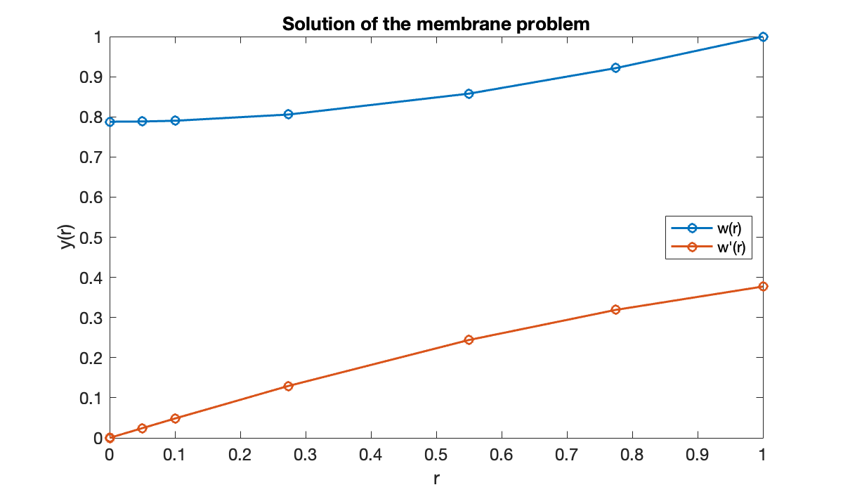

It’s smart to check visually that the boundary conditions are satisfied.

10.2 Shooting¶

Example 10.2.1

Let’s first examine the shooting approach for the TPBVP from Example 10.1.2 with $\lambda=0.6$ .

lambda = 0.6;
phi = @(r, w, dwdr) lambda ./ w.^2 - dwdr ./ r;

We convert the ODE to a first-order system in order to apply a numerical method. We also have to truncate the domain to avoid division by zero.

f = @(r, w) [ w(2); phi(r, w(1), w(2)) ];
a = eps;  b = 1;

The BVP specifies $w'(0)=y_2(0)=0$ . We can try multiple values for the unknown $w(0)=y_1(0)$ and plot the solutions.

clf
ivp = ode;
ivp.ODEFcn = f;
ivp.InitialTime = a;
for w0 = 0.4:0.1:0.9
    ivp.InitialValue = [w0; 0];
    sol = solve(ivp, a, b);
    plot(sol.Time, sol.Solution(1, :))
    hold on
end
xlabel('r'),  ylabel('w(r)')
title('Solutions for multiple choices of w(0)')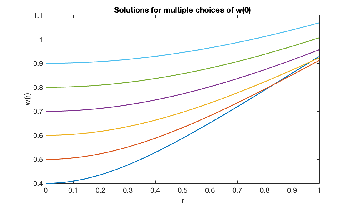

On the graph, it’s the curve starting at $w(0)=0.8$ that comes closest to the required condition $w(1)=1$ , but it’s a bit too large.

Example 10.2.2

We revisit Demo 10.2.1 but let Function 10.2.1 do the heavy lifting.

lambda = 0.6;
phi = @(r, w, dwdr) lambda ./ w.^2 - dwdr ./ r;   
a = eps;  b = 1;    % avoid r=0 in denominator

We specify the given and unknown endpoint values.

ga = @(u, du) du;
gb = @(u, du) u - 1;

init = [0.8; 0];    % initial guess for u(a) and u'(a)
[r, w, dwdx] = shoot(phi, a, b, ga, gb, init, 1e-5);
clf,  plot(r, w)
title('Correct solution')
xlabel('r'),  ylabel('w(r)')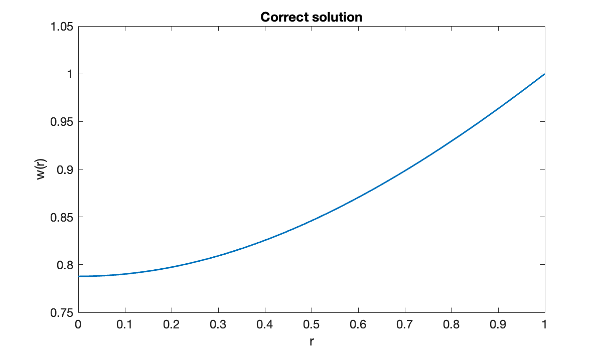

The value of $w$ at $r=1$ , meant to be exactly one, was computed to be

format long
w(end)

The accuracy is consistent with the error tolerance used for the IVP solution. The initial value $w(0)$ that gave this solution is

w(1)

Example 10.2.3

ga = @(u, du) u + 1;
gb = @(u, du) u;
clf
warning off
for lambda = 16:4:28
    phi = @(x, u, du_dx) lambda^2 * (u + 1);
    [x, u, du_dx] = shoot(phi, 0.0, 1.0, ga, gb, [-1; 0], 1e-8);
    plot(x, u, displayname=sprintf("lambda=%d", lambda))
    hold on
    xlabel('x'),  ylabel('u(x)')
    title('Shooting instability')
    legend(location="northwest");
end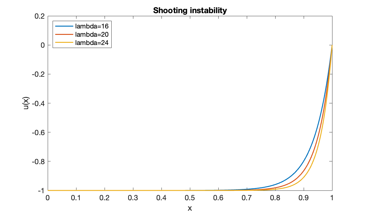

Error using shoot/objective (line 27)
Error setting property 'InitialValue' of class 'ode'. Value must be finite.

Error in levenberg (line 27)
    xnew = x(:,k) + s;   fnew = f(xnew);

Error in shoot (line 34)
s = levenberg(@objective, init, tol);

The numerical solution fails at the largest value of λ because the initial condition became infinite.

10.3 Differentiation matrices¶

Example 10.3.1

We test first-order and second-order differentiation matrices for the function $x + \exp(\sin 4x)$ over $[-1,1]$ .

f = @(x) x + exp(sin(4*x));

For reference, here are the exact first and second derivatives.

df_dx = @(x) 1 + 4 * exp(sin(4*x)) .* cos(4*x);
d2f_dx2 = @(x) 4 * exp(sin(4*x)) .* (4*cos(4*x).^2 - 4*sin(4*x));

We discretize on equally spaced nodes and evaluate $f$ at the nodes.

[t, Dx, Dxx] = diffmat2(12, [-1 1]);
y = f(t);

Then the first two derivatives of $f$ each require one matrix-vector multiplication.

yx = Dx * y;
yxx = Dxx * y;

The results show poor accuracy for this small value of $n$ .

clf,  subplot(2, 1, 1)
fplot(df_dx, [-1, 1]),  hold on
plot(t, yx, 'ko')
xlabel('x'),  ylabel('f''(x)')
subplot(2, 1, 2)
fplot(d2f_dx2, [-1, 1]),  hold on
plot(t, yxx, 'ko')
xlabel('x'),  ylabel('f''''(x)')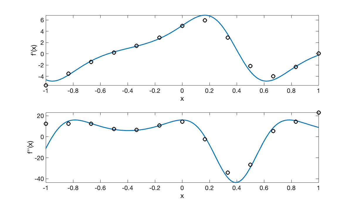

An convergence experiment confirms the order of accuracy. Because we expect an algebraic convergence rate, we use a log-log plot of the errors.

n = round( 2 .^ (4:.5:11)' );
err = zeros(length(n), 2);
for k = 1:length(n)
    [t, Dx, Dxx] = diffmat2(n(k), [-1, 1]);
    y = f(t);
    err(k, 1) = norm(df_dx(t) - Dx * y, Inf);
    err(k, 2) = norm(d2f_dx2(t) - Dxx * y, Inf);
end
clf
loglog(n, err, 'o-'), hold on
loglog(n, 100 * n.^(-2), 'k--')
legend("f'", "f''", '2nd order')
xlabel('n'),  ylabel('max error')
title('Convergence of finite differences')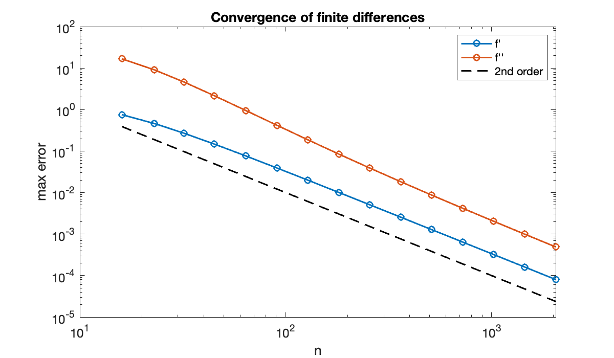

Example 10.3.2

Here is a $4\times 4$ Chebyshev differentiation matrix.

[t, Dx] = diffcheb(3, [-1, 1]);
format rat
Dx

We again test the convergence rate.

f = @(x) x + exp(sin(4*x));
df_dx = @(x) 1 + 4 * exp(sin(4*x)) .* cos(4*x);
d2f_dx2 = @(x) 4 * exp(sin(4*x)) .* (4*cos(4*x).^2 - 4*sin(4*x));

n = 5:5:70;
err = zeros(length(n), 2);
for k = 1:length(n)
    [t, Dx, Dxx] = diffcheb(n(k), [-1, 1]);
    y = f(t);
    err(k, 1) = norm(df_dx(t) - Dx * y, Inf);
    err(k, 2) = norm(d2f_dx2(t) - Dxx * y, Inf);
end

Since we expect a spectral convergence rate, we use a semi-log plot for the error.

clf,  format
semilogy(n, err, 'o-'), hold on
legend("f'", "f''")
xlabel('n'),  ylabel('max error')
title('Convergence of finite differences')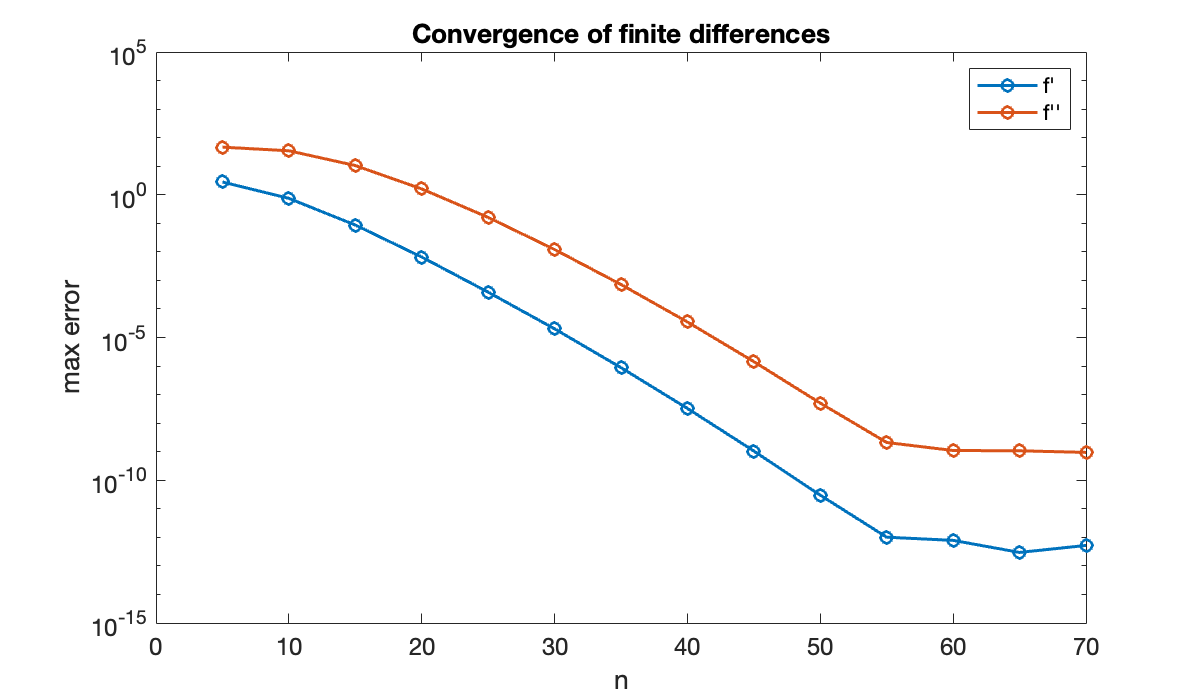

10.4 Collocation for linear problems¶

Example 10.4.1

exact = @(x) exp(sin(x));

The problem is presented above in our standard form, so we can identify the coefficient functions in the ODE. Each should be coded as a function.

p = @(x) -cos(x);
q = @(x) sin(x);
r = @(x) 0*x;      % not a scalar

We solve the BVP and compare the result to the exact solution.

[x, u] = bvplin(p, q, r, 0, 3*pi/2, 1, exp(-1), 30);

clf,  subplot(2, 1, 1)
plot(x, u)
ylabel('solution')
title('Solution of a linear BVP')
subplot(2, 1, 2)
plot(x, exact(x) - u, 'o-')
ylabel('error')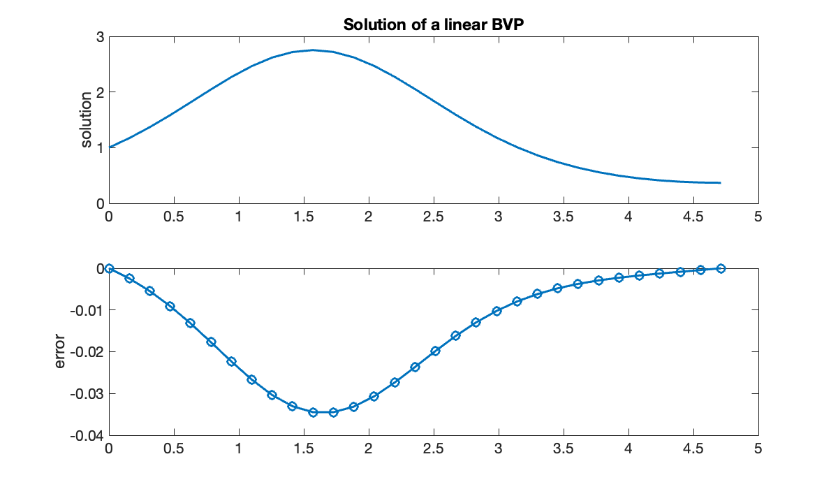

Example 10.4.2

lambda = 10;
exact = @(x) sinh(lambda * x) / sinh(lambda) - 1;

The following functions define the ODE.

p = @(x) zeros(size(x));            
q = @(x) -lambda^2 * ones(size(x));
r = @(x) lambda^2 * ones(size(x));

We compare the computed solution to the exact one for increasing $n$ .

p = @(x) zeros(size(x));            
q = @(x) -lambda^2 * ones(size(x));
r = @(x) lambda^2 * ones(size(x));
n = 2 * round(10.^(1:0.25:3)');
err = zeros(size(n));
for k = 1:length(n)
    [x, u] = bvplin(p, q, r, 0, 1, -1, 0, n(k));
    err(k) = norm(exact(x) - u, Inf);
end
disp(table(n, err, variableNames = ["n", "inf-norm error"]))

     n      inf-norm error

    ____    ______________

      20       0.0037471

      36       0.0011679

      64      0.00037262

     112      0.00012209

     200      3.8312e-05

     356      1.2093e-05

     632      3.8375e-06

    1124      1.2133e-06

    2000      3.8321e-07

Each factor of 10 in $n$ reduces error by a factor of 100, which is indicative of second-order convergence.

clf,  loglog(n, err, 'o-')
hold on, loglog(n, n.^(-2), 'k--')
xlabel('n'),  ylabel('max error')
title('Convergence for a linear BVP') 
legend('obs. error', '2nd order')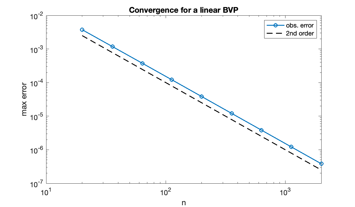

10.5 Nonlinearity and boundary conditions¶

Example 10.5.2

Suppose a damped pendulum satisfies the nonlinear equation $\theta'' + 0.05\theta'+\sin \theta =0$ . We want to start the pendulum at $\theta=2.5$ and give it the right initial velocity so that it reaches $\theta=-2$ at exactly $t=5$ . This is a boundary-value problem with Dirichlet conditions $\theta(0)=2.5$ and $\theta(5)=-2$ .

The first step is to define the function ϕ that equals $\theta''$ .

phi = @(t,theta,omega) -0.05 * omega - sin(theta);

Next, we define the boundary conditions.

ga = @(u, du) u - 2.5;
gb = @(u, du) u + 2;

The last ingredient is an initial estimate of the solution. Here we choose $n=100$ and a linear function between the endpoint values.

init = linspace(2.5, -2, 101)';

We find a solution with negative initial slope, i.e., the pendulum is initially pushed back toward equilibrium.

[t, theta] = bvp(phi, 0, 5, ga, gb, init);
clf,  plot(t, theta)
xlabel('t'),  ylabel('\theta(t)')
title('Pendulum over [0,5]')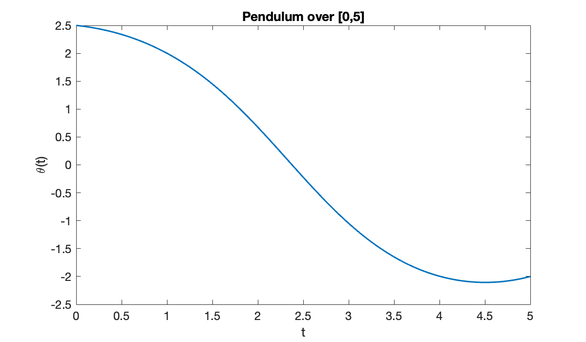

If we extend the time interval longer for the same boundary values, then the initial slope must adjust.

[t, theta] = bvp(phi, 0, 8, ga, gb, init);
plot(t,theta)
xlabel('t'),  ylabel('\theta(t)')
title('Pendulum over [0,8]')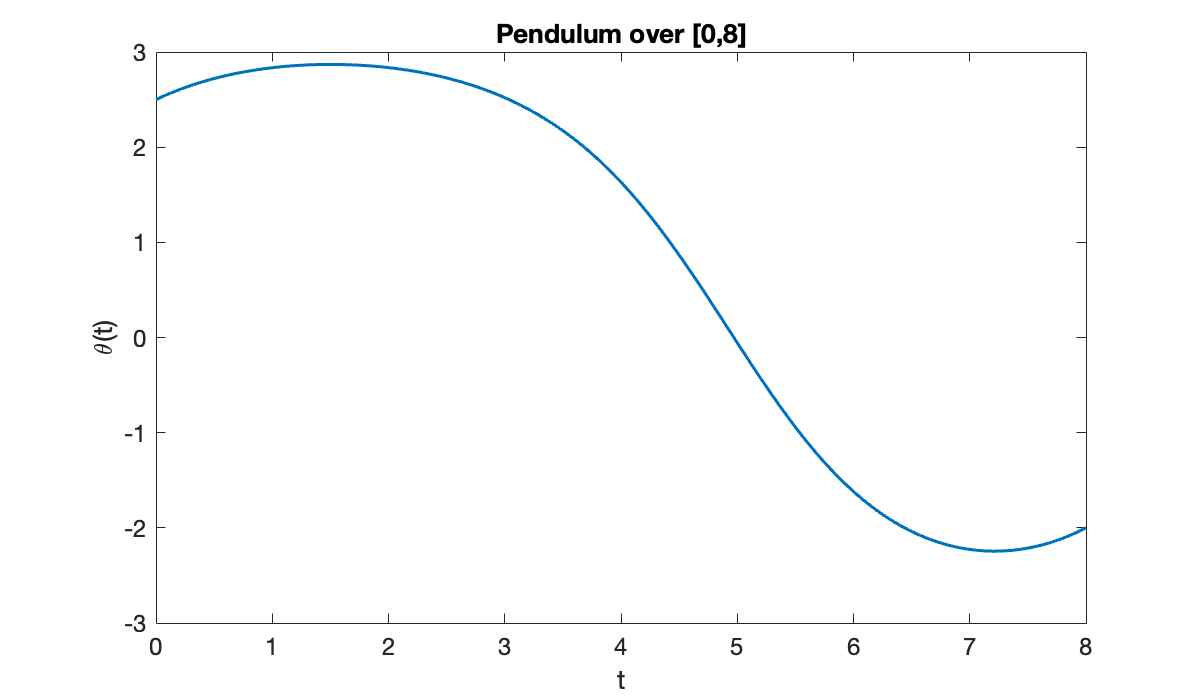

This time, the pendulum is initially pushed toward the unstable equilibrium in the upright vertical position before gravity pulls it back down.

Example 10.5.3

Here is the problem definition. We use a truncated domain to avoid division by zero at $r=0$ .

lambda = 0.5;
phi = @(r,w,dwdr) lambda./w.^2 - dwdr./r;
ga = @(w, dw) dw;
gb = @(w, dw) w - 1;
a = eps;  b = 1;

First we try a constant function as the initialization.

init = ones(301, 1);
[r, w1] = bvp(phi, a, b, ga, gb, init);

clf,  plot(r, w1)
xlabel('r'),  ylabel('w(r)')
title('Solution of the MEMS BVP')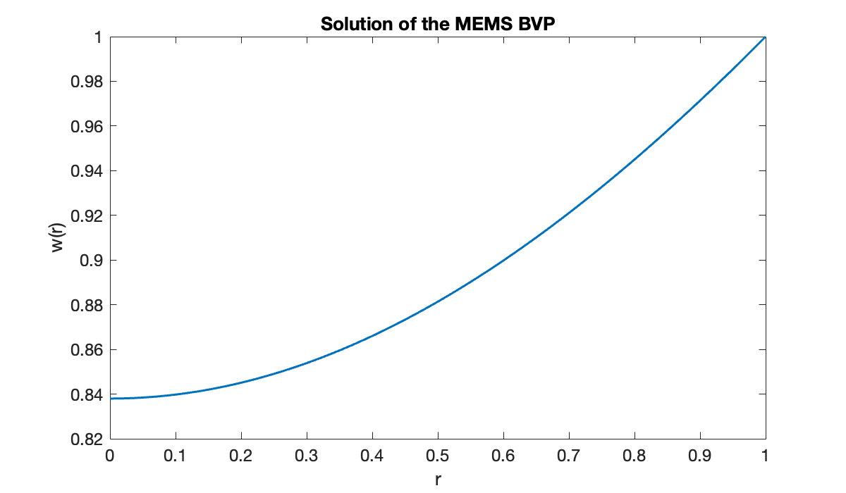

It’s not necessary that the initialization satisfy the boundary conditions. In fact, by choosing a different constant function as the initial guess, we arrive at another valid solution.

init = 0.5 * ones(301, 1);
[r, w2] = bvp(phi, a, b, ga, gb, init);
hold on,  plot(r, w2)
title("Two solutions of the MEMS BVP")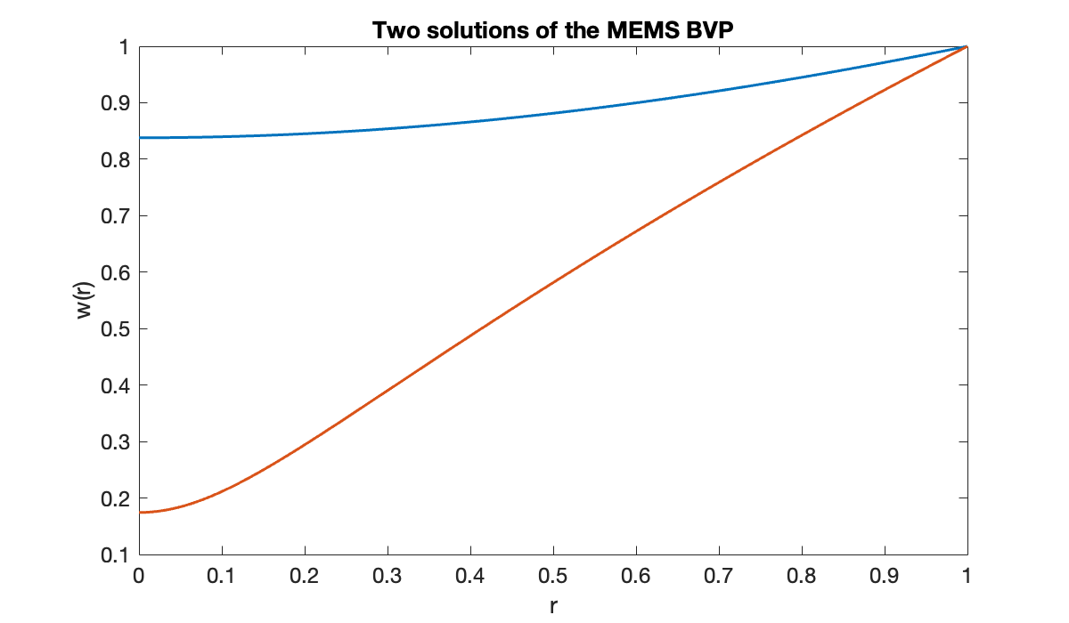

Example 10.5.4

epsilon = 0.05;
phi = @(x, u, du_dx) (u.^3 - u) / epsilon;
ga = @(u, du) du;
gb = @(u, du) u - 1;

Finding a solution is easy at larger values of ε.

init = linspace(-1, 1, 141)';
[x, u1] = bvp(phi, 0, 1, ga, gb, init);
clf,  plot(x, u1, displayname="\epsilon = 0.05")
xlabel('x'),  ylabel('u(x)')
title('Allen-Cahn solution') 
legend(location="northwest")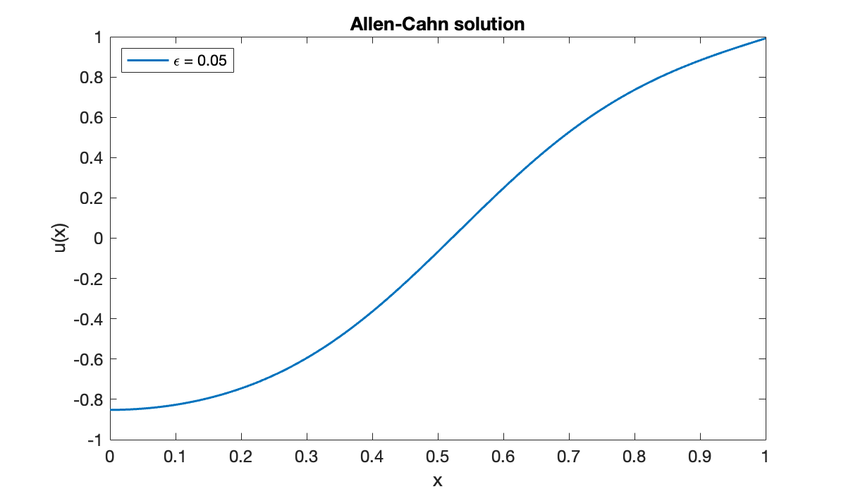

However, finding a good initialization is not trivial for smaller values of ε. Note below that the iteration stops without converging to a solution.

epsilon = 0.002;
phi = @(x, u, du_dx) (u.^3 - u) / epsilon;
[x, z] = bvp(phi, 0, 1, ga, gb, init);

The iteration succeeds if we use the first solution instead as the initialization here.

[x, u2] = bvp(phi, 0, 1, ga, gb, u1);
hold on,  plot(x, u2, displayname="\epsilon = 0.002")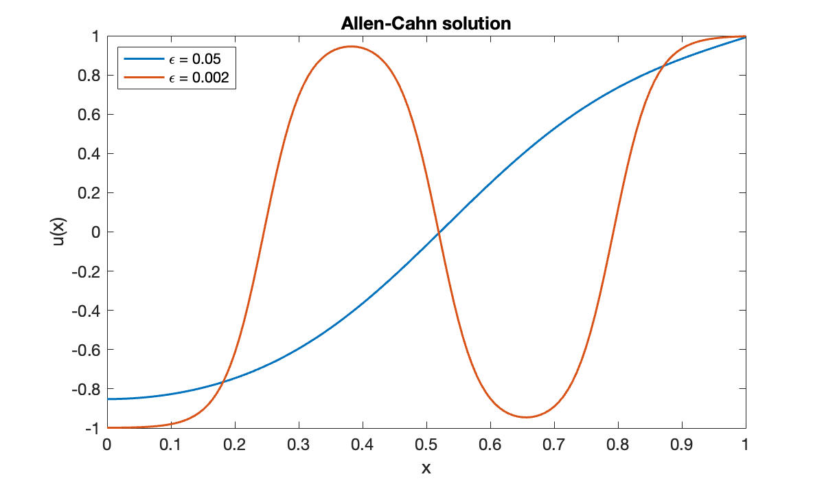

In this case we can continue further.

epsilon = 0.0005;
phi = @(x, u, du_dx) (u.^3 - u) / epsilon;
[x, u3] = bvp(phi, 0, 1, ga, gb, u2);
plot(x, u3, displayname="\epsilon = 0.0005")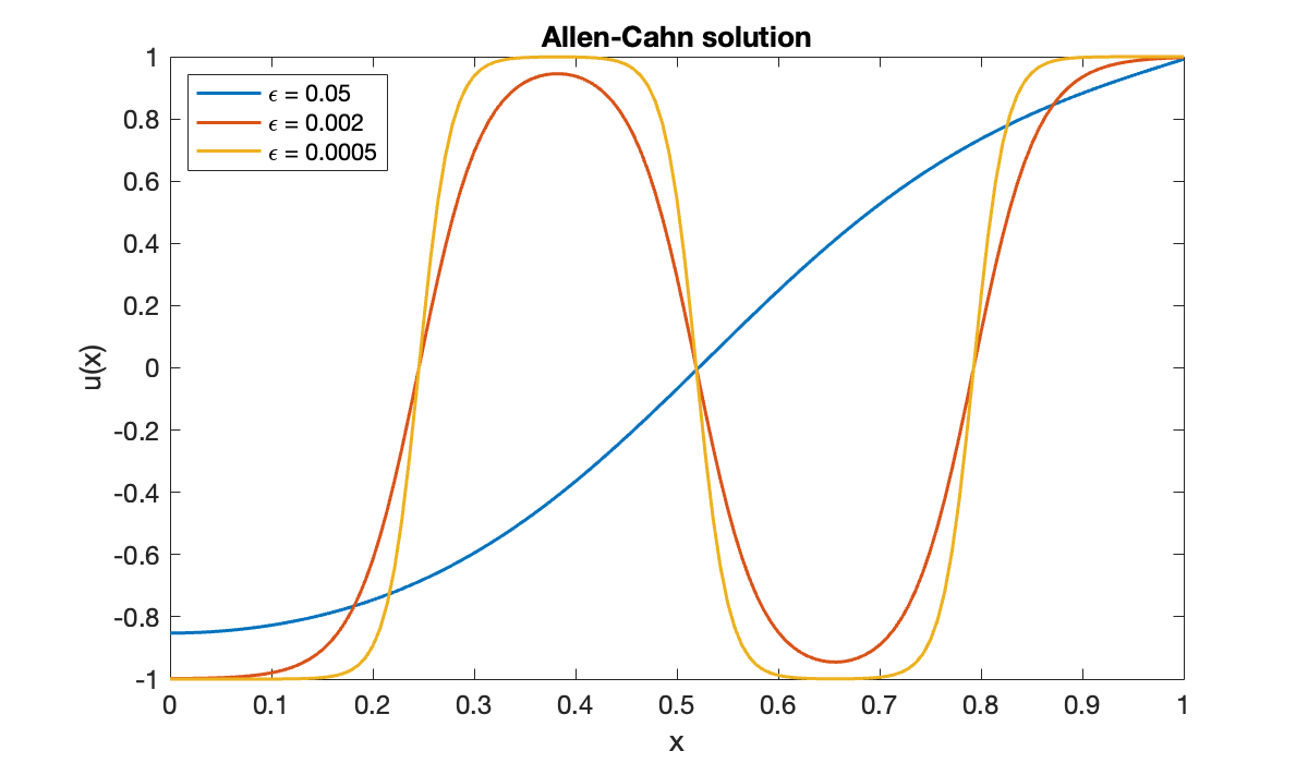

10.6 The Galerkin method¶

Example 10.6.2

Here are the coefficient function definitions. Even though $s$ is a constant, it has to be defined as a function for Function 10.6.1 to use it.

c = @(x) x.^2;
q = @(x) 4 * ones(size(x));
f = @(x) sin(pi * x);

[x,u] = fem(c, q, f, 0, 1, 50);
clf,  plot(x, u)
xlabel('x'),  ylabel('u')
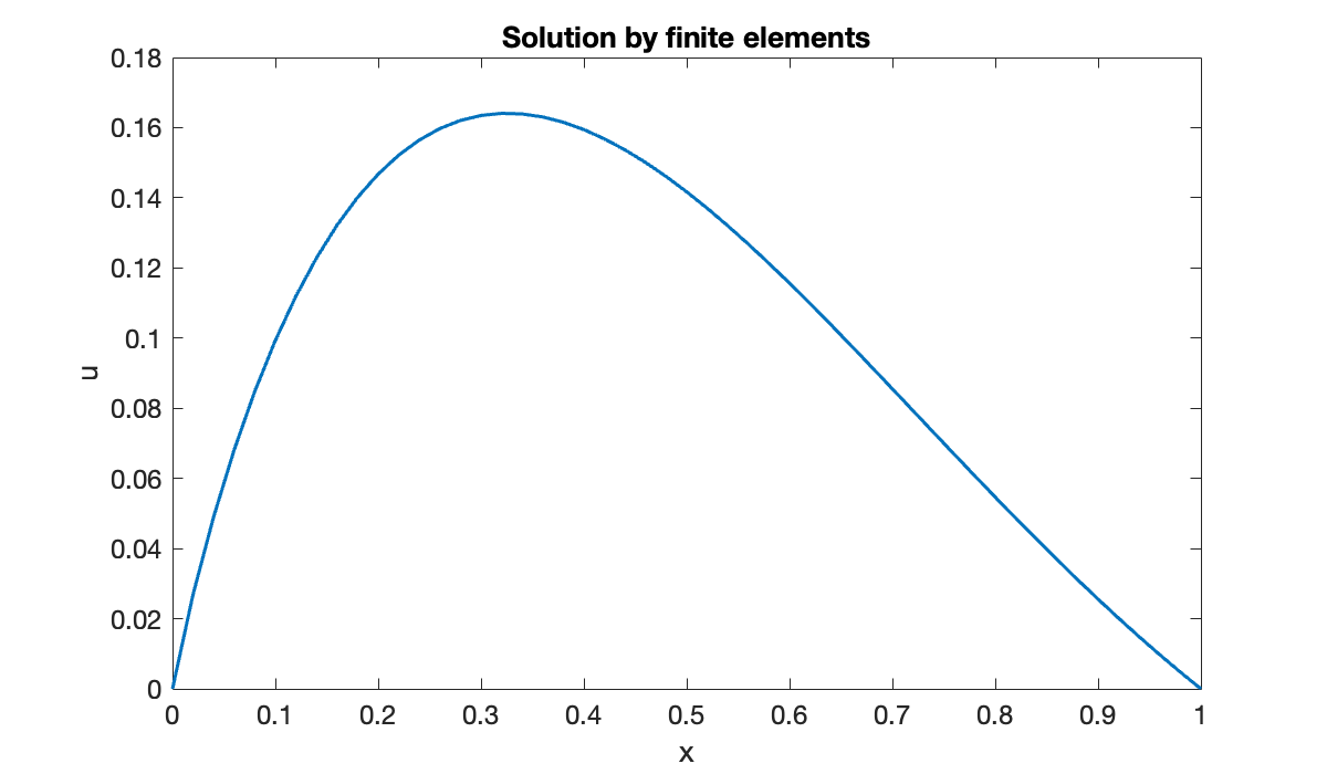
title('Solution by finite elements')