Chapter 9 - Fundamentals of Numerical Computation

Functions¶

Barycentric polynomial interpolation

polyinterp.m

1
2
3
4
5
6
7
8
9
10
11
12
13
14
15
16
17
18
19
20
21
22
23
24
25
26
27
28
29
30
31
32
33
34
35
36
37
38
39
40
function p = polyinterp(t,y)
% POLYINTERP Polynomial interpolation by the barycentric formula.
% Input:
%   t   interpolation nodes (vector, length n+1)
%   y   interpolation values (vector, length n+1)
% Output:
%   p   polynomial interpolant (function)

t = t(:);                    % column vector
n = length(t)-1;
C = (t(end)-t(1)) / 4;       % scaling factor to ensure stability
tc = t/C;

% Adding one node at a time, compute inverses of the weights.
omega = ones(n+1,1);
for m = 1:n
    d = (tc(1:m) - tc(m+1));    % vector of node differences
    omega(1:m) = omega(1:m).*d; % update previous 
    omega(m+1) = prod( -d );    % compute the new one
end
w = 1./omega;                   % go from inverses to weights

p = @evaluate;

    function f = evaluate(x)
        % % Compute interpolant, one value of x at a time.
        f = zeros(size(x));
        for j = 1:numel(x)
            terms = w ./ (x(j) - t );
            f(j) = sum(y.*terms) / sum(terms);
        end
        
        % Apply L'Hopital's Rule exactly.
        for j = find( isnan(f(:)) )'      % divided by zero here
            [~,idx] = min( abs(x(j)-t) );   % node closest to x(j)
            f(j) = y(idx);                  % value at node
        end        
    end

end

Trigonometric interpolation

triginterp.m

1
2
3
4
5
6
7
8
9
10
11
12
13
14
15
16
17
18
19
20
21
22
23
24
25
26
27
28
function p = triginterp(t,y)
% TRIGINTERP Trigonometric interpolation.
% Input:
%   t   equispaced interpolation nodes (vector, length N)
%   y   interpolation values (vector, length N)
% Output:
%   p   trigonometric interpolant (function)

N = length(t);
p = @value;

    function f = value(x)
        f = zeros(size(x));
        for k = 1:N
            f = f + y(k)*trigcardinal(x-t(k));
        end
    end
        
    function tau = trigcardinal(x)
        if rem(N,2)==1   % odd
            tau = sin(N*pi*x/2) ./ (N*sin(pi*x/2));
        else             % even
            tau = sin(N*pi*x/2) ./ (N*tan(pi*x/2));
        end
        tau(isnan(tau)) = 1;
    end
        
end

Clenshaw-Curtis integration

ccint.m

1
2
3
4
5
6
7
8
9
10
11
12
13
14
15
16
17
18
19
20
21
22
23
24
25
26
function [I,x] = ccint(f,n)
% CCINT  Clenshaw-Curtis numerical integration.
% Input:
%   f     integrand (function)
%   n     one less than the number of nodes (even integer)
% Output:
%   I     estimate of integral(f,-1,1)
%   x     evaluation nodes of f (vector)

% Find Chebyshev extreme nodes.
theta = pi*(0:n)'/n;
x = -cos(theta);

% Compute the C-C weights.
c = zeros(1,n+1); 
c([1 n+1]) = 1/(n^2-1); 
theta = theta(2:n); 
v = ones(n-1,1);
for k = 1:n/2-1
  v = v - 2*cos(2*k*theta)/(4*k^2-1);
end
v = v - cos(n*theta)/(n^2-1);
c(2:n) = 2*v/n;

% Evaluate integrand and integral.
I = c*f(x);   % use vector inner product

Gauss-Legendre integration

glint.m

1
2
3
4
5
6
7
8
9
10
11
12
13
14
15
16
17
18
function [I,x] = glint(f,n)
% GLINT  Gauss-Legendre numerical integration.
% Input:
%   f     integrand (function)
%   n     number of nodes (integer)
% Output:
%   I     estimate of integral(f,-1,1)
%   x     evaluation nodes of f (vector)

% Nodes and weights are found via a tridiagonal eigenvalue problem.
beta = 0.5./sqrt(1-(2*(1:n-1)).^(-2));
T = diag(beta,1) + diag(beta,-1);
[V,D] = eig(T);
x = diag(D); [x,idx] = sort(x);    % nodes
c = 2*V(1,idx).^2;                 % weights

% Evaluate the integrand and compute the integral.
I = c*f(x);      % vector inner product

Integration over

(-\infty,\infty)

intinf.m

1
2
3
4
5
6
7
8
9
10
11
12
13
14
15
16
17
18
19
20
21
22
23
24
25
26
27
function [I, x] = intinf(f, tol)
% INTINF   Adaptive doubly exponential integration over (-inf,inf).
% Input:
%   f   integrand (function)
%   tol error tolerance (positive scalar)
% Output:
%   I   approximation to intergal(f) over (-inf,inf)
%   x   evaluation nodes (vector) 

xi = @(t) sinh(sinh(t));
dxi_dt = @(t) cosh(t) .* cosh(sinh(t));
g = @(t) f(xi(t)) .* dxi_dt(t);

% Find where to truncate the integration interval.
M = 3;
while (abs(g(-M)) > tol/100) || (abs(g(M)) > tol/100)
    M = M + 0.5;
    if isinf(xi(M)) 
        warning("Function may not decay fast enough.")
        M = M - 0.5;
        break
    end
end

[I, t] = intadapt(g, -M, M, tol);
x = xi(t);
end

Integration with endpoint singularities

intsing.m

1
2
3
4
5
6
7
8
9
10
11
12
13
14
15
16
17
18
19
20
21
22
23
24
25
26
27
function [I, x] = intsing(f, tol)
% INTSING   Adaptively integrate a function with a singularity at the left endpoint.
% Input:
%   f   integrand  (function)
%   tol error tolerance (positive scalar)
% Output:
%   I   approximation to integral(f) over (0,1)
%   x   evaluation nodes (vector)

xi = @(t) 2 ./ (1 + exp( 2*sinh(t) ));
dxi_dt = @(t) cosh(t) ./ cosh( sinh(t) ).^2;
g = @(t) f(xi(t)) .* dxi_dt(t);

% Find where to truncate the integration interval.
M = 3;
while abs(g(M)) > tol/100
    M = M + 0.5;
    if xi(M) == 0
        warning("Function may grow too rapidly.")
        M = M - 0.5;
        break
    end
end

[I, t] = intadapt(g, 0, M, tol);
x = xi(t);
end

Examples¶

9.1 Polynomial interpolation¶

Example 9.1.1

Here is a vector of nodes.

t = [ 1, 1.5, 2, 2.25, 2.75, 3 ];
n = 5;  k = 2;
not_k = [0:k-1 k+1:n];   % all except the kth node

Let’s apply the definition of the cardinal Lagrange polynomial for $k=2$ . First we define a polynomial $q$ that is zero at all the nodes except $i=k$ . Then $\ell_2$ is found by normalizing $q$ by $q(t_k)$ .

q = @(x) prod(x - t(not_k + 1));
ell_k = @(x) q(x) ./ q(t(k + 1));

A plot confirms the cardinal property of the result.

clf
fplot(ell_k, [1, 3])
hold on, grid on
plot(t(not_k + 1), 0 * t(not_k + 1), 'o')
plot(t(k + 1), 1, 'o')
xlabel('x'),  ylabel('\ell_2(x)')    
title('Lagrange cardinal function')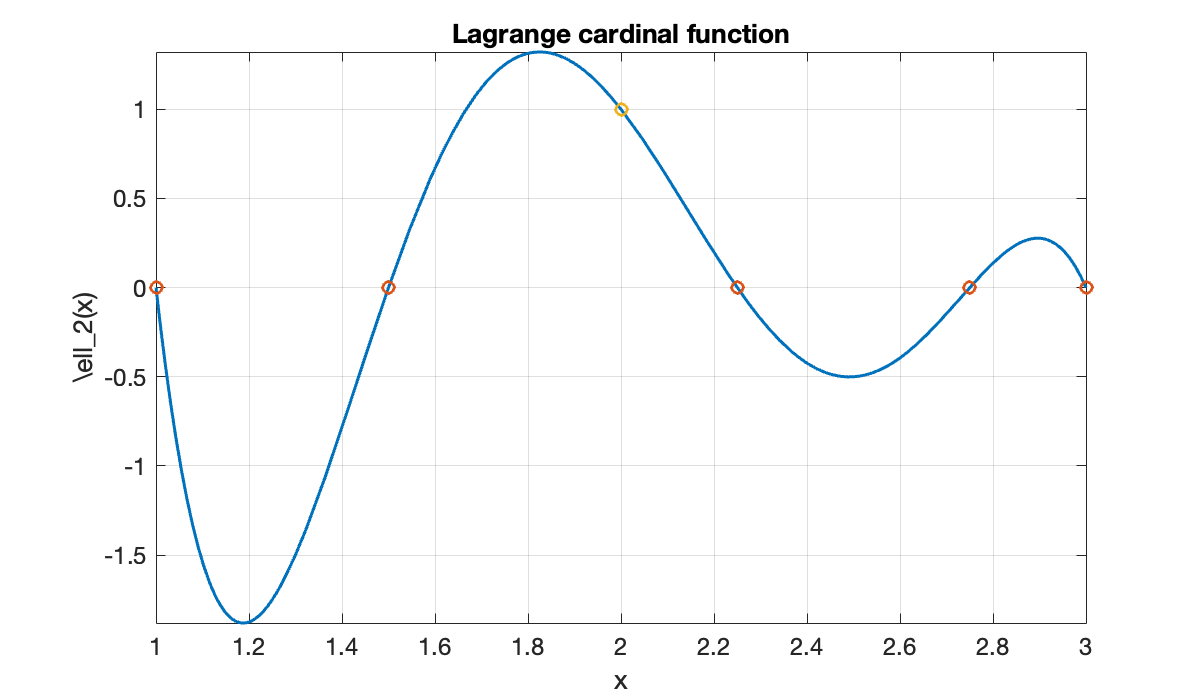

Observe that $\ell_k$ is not between zero and one everywhere, unlike a hat function.

Example 9.1.3

t =  [ 1, 1.6, 1.9, 2.7, 3 ];
n = length(t) - 1;
Phi = @(x) prod(x - t);

clf,  fplot(@(x) Phi(x) / 5, [1, 3])
hold on,  plot(t, 0*t, 'o')
xlabel('x'),  ylabel('\Phi(x)')   
title('Interpolation error function')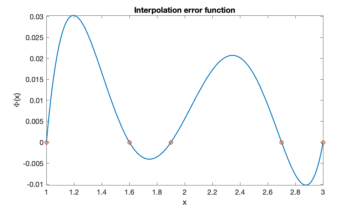

The error is zero at the nodes, by the definition of interpolation. The error bound, as well as the error itself, has one local maximum between each consecutive pair of nodes.

9.2 The barycentric formula¶

Example 9.2.2

f = @(x) sin( exp(2 * x) );
clf,  fplot(f, [0, 1], displayname="function")
xlabel('x'),  ylabel('f(x)')   
legend(location="southwest");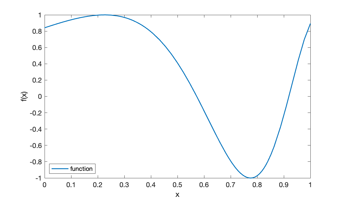

We start with 4 equally spaced nodes ( $n=3$ ).

t = linspace(0, 1, 4)'; 
y = f(t);
p = polyinterp(t, y);
hold on,  fplot(p, [0, 1], displayname="interpolant on 4 nodes")
scatter(t, y, 'k', displayname="nodes")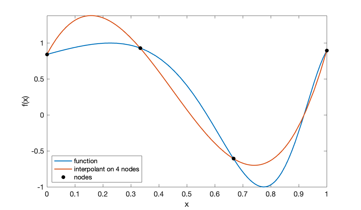

The curves always intersect at the interpolation nodes. For $n=6$ , the interpolant is noticeably better.

cla,  fplot(f, [0, 1], displayname="function")
t = linspace(0, 1, 7)'; 
y = f(t);
p = polyinterp(t, y);
hold on,  fplot(p, [0, 1], displayname="interpolant on 7 nodes")
scatter(t, y, 'k', displayname="nodes")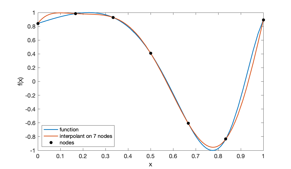

9.3 Stability of polynomial interpolation¶

Example 9.3.1

We choose a function over the interval $[0,1]$ . Using 7 equally spaced nodes, the interpolation looks fine.

f = @(x) sin(exp(2*x));
clf,  fplot(f, [0, 1], displayname="function")
t = linspace(0, 1, 7);
y = f(t);
hold on,  scatter(t, y, displayname="nodes")
p = polyinterp(t, y)
fplot(p, [0, 1], displayname="interpolant")
xlabel('x'),  ylabel('f(x)') 
title('Test function')

We want to track the behavior of the error as $n$ increases. We will estimate the error in the continuous interpolant by sampling it at a large number of points and taking the max-norm.

n = (5:5:60)';   
err = zeros(size(n));
x = linspace(0, 1, 1001)';         % for measuring error
for k = 1:length(n) 
  t = linspace(0, 1, n(k) + 1)';     % equally spaced nodes
  y = f(t);                      % interpolation data
  p = polyinterp(t, y);
  err(k) = norm(f(x) - p(x), Inf);
end
clf,  semilogy(n, err, 'o-')
xlabel('n'),  ylabel('max error')   
title('Equispaced polynomial interpolation error')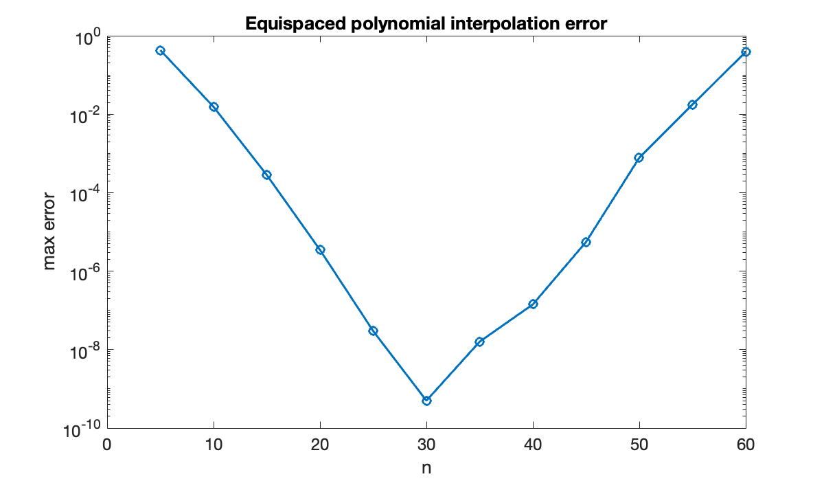

The error initially decreases as one would expect but then begins to grow. Both phases occur at rates that are exponential in $n$ , i.e., $O(K^n$ ) for a constant $K$ , appearing linear on a semi-log plot.

Example 9.3.2

We plot $|\Phi(x)|$ over the interval $[-1,1]$ with equispaced nodes for different values of $n$ .

clf
x = linspace(-1, 1, 1601)';
Phi = zeros(size(x));
for n = 10:10:50
    t = linspace(-1, 1, n+1)';
    for k = 1:length(x)
        Phi(k) = prod(x(k) - t);
    end
    semilogy(x, abs(Phi)),  hold on
end
title('Error indicator on equispaced nodes')    
xlabel('x'),  ylabel('|\Phi(x)|')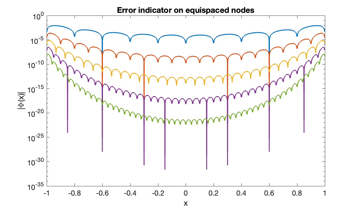

Each time Φ passes through zero at an interpolation node, the value on the log scale should go to $-\infty$ , which explains the numerous cusps on the curves.

Example 9.3.3

This function has infinitely many continuous derivatives on the entire real line and looks easy to approximate over $[-1,1]$ .

f = @(x) 1 ./ (x.^2 + 16);
clf,  fplot(f, [-1, 1])
xlabel('x'),  ylabel('f(x)')    
title('Test function')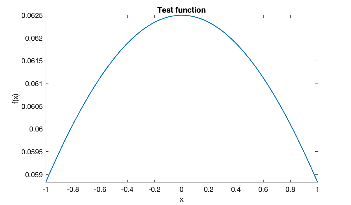

We start by doing equispaced polynomial interpolation for some small values of $n$ .

x = linspace(-1, 1, 1601)';
n = (4:4:12)';
for k = 1:length(n)
    t = linspace(-1, 1, n(k) + 1)';        % equally spaced nodes
    p = polyinterp(t, f(t));
    semilogy(x, abs(f(x) - p(x)));  hold on
end
title('Error for degrees 4, 8, 12')   
xlabel('x'), ylabel('|f(x) - p(x)|')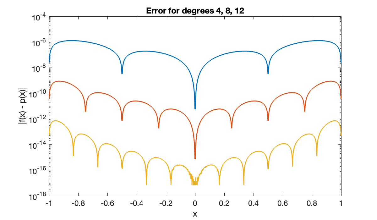

The convergence so far appears rather good, though not uniformly so. However, notice what happens as we continue to increase the degree.

n = 12 + 15 * (1:3);
clf
for k = 1:length(n)
    t = linspace(-1, 1, n(k) + 1)';        % equally spaced nodes
    p = polyinterp(t, f(t));
    semilogy(x, abs(f(x) - p(x)));  hold on
end
title('Error for degrees 27, 42, 57')   
xlabel('x'), ylabel('|f(x) - p(x)|')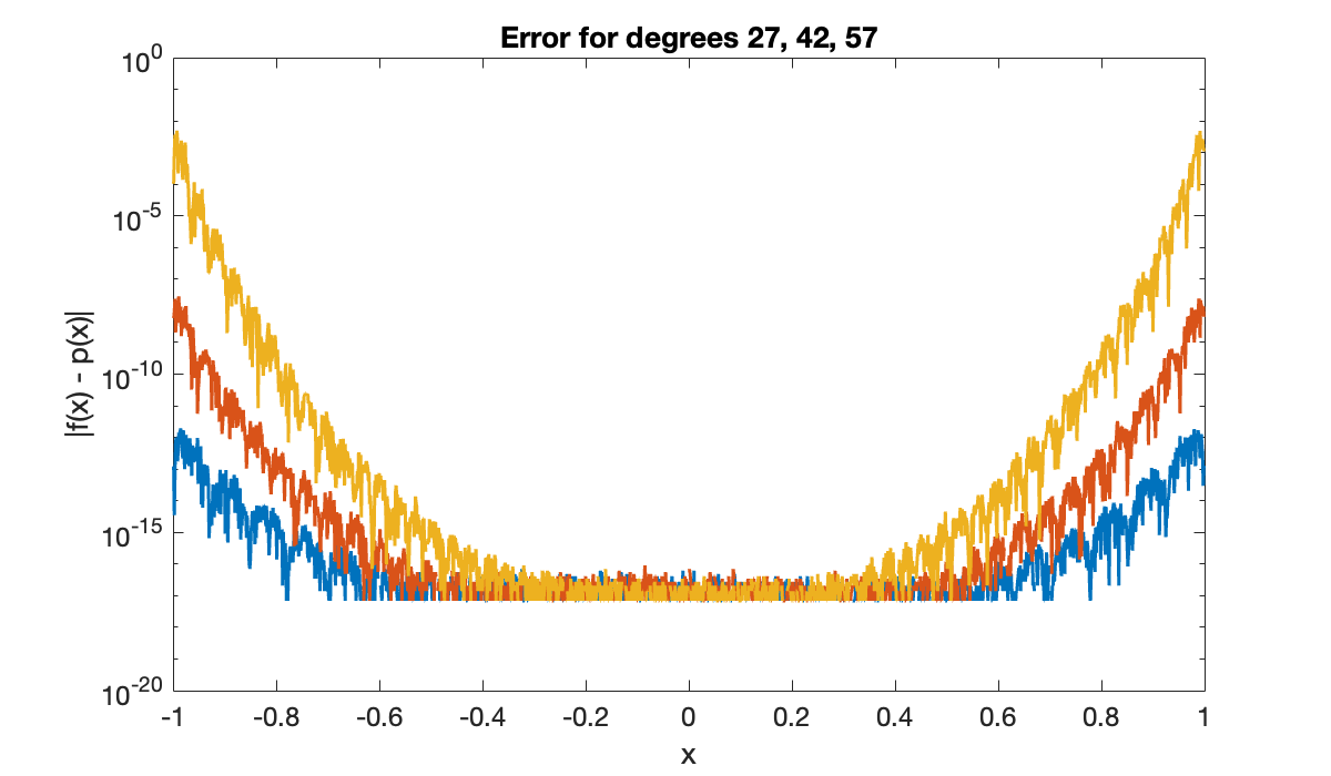

The convergence in the middle can’t get any better than machine precision relative to the function values. So maintaining the growing gap between the center and the ends pushes the error curves upward exponentially fast at the ends, wrecking the convergence.

Example 9.3.4

Now we look at the error indicator function Φ for Chebyshev node sets.

clf
x = linspace(-1, 1, 1601)';
Phi = zeros(size(x));
for n = 10:10:50
    theta = linspace(0, pi, n+1)';
    t = -cos(theta);                    
    for k = 1:length(x)
        Phi(k) = prod(x(k) - t);
    end
    semilogy(x, abs(Phi));  hold on
end
axis tight, title('Effect of Chebyshev nodes')    
xlabel('x'), ylabel('|\Phi(x)|')   
ylim([1e-18, 1e-2])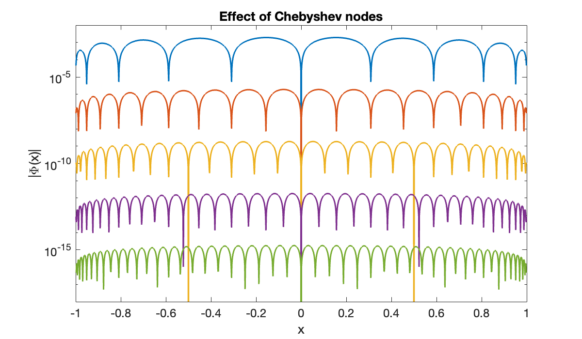

In contrast to the equispaced case, $|\Phi|$ decreases exponentially with $n$ almost uniformly across the interval.

Example 9.3.5

Here again is the function from Demo 9.3.3 that provoked the Runge phenomenon when using equispaced nodes.

f = @(x) 1 ./ (x.^2 + 16);

clf
x = linspace(-1, 1, 1601)';
n = [4, 10, 16, 40];
for k = 1:length(n) 
    theta = linspace(0, pi, n(k) + 1)';
    t = -cos(theta);
    p = polyinterp(t, f(t));
    semilogy( x, abs(f(x) - p(x)) );  hold on
end
title('Error for degrees 4, 10, 16, 40')   
xlabel('x'), ylabel('|f(x)-p(x)|')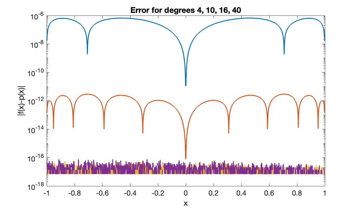

By degree 16 the error is uniformly within machine epsilon, and, importantly, it stays there as $n$ increases. Note that as predicted by the error indicator function, the error is uniform over the interval at each value of $n$ .

Example 9.3.6

On the left, we use a log-log scale, which makes second-order algebraic convergence $O(n^{-4})$ a straight line. On the right, we use a log-linear scale, which makes spectral convergence $O(K^{-n})$ linear.

n = (20:20:400)';
algebraic = 100 ./ n.^4;
spectral = 10 * 0.85.^n;
clf, subplot(2, 1, 1)
loglog(n, algebraic, 'o-', displayname="algebraic")
hold on;  loglog(n, spectral, 'o-', displayname="spectral")
xlabel('n'),  ylabel('error')   
title('log–log')   
axis tight,  ylim([1e-16, 1]);  legend(location="southwest")   

subplot(2, 1, 2)
semilogy(n, algebraic, 'o-', displayname="algebraic")
hold on;  semilogy(n, spectral, 'o-', displayname="spectral")
xlabel('n'), ylabel('error'),  ylim([1e-16, 1])   
title('log–linear')   
axis tight,  ylim([1e-16, 1]);  legend(location="southwest")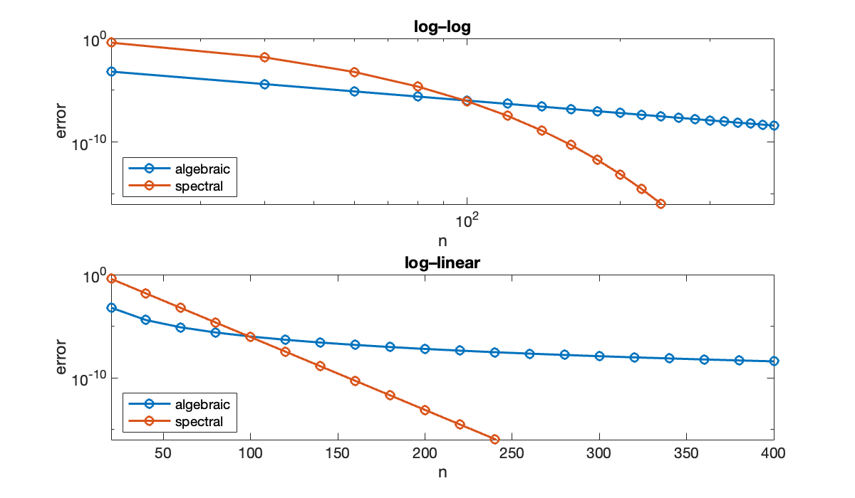

9.4 Orthogonal polynomials¶

Example 9.4.1

Let’s approximate $e^x$ over the interval $[−1,1]$ . We can sample it at, say, 15 points, and find the best-fitting straight line to that data.

clf;  fplot(@exp, [-1, 1], displayname="function")
t = linspace(-1, 1, 15)';
y = exp(t);
V = [t.^0, t];
c = V \ y;
p = @(t) c(1) + c(2)*t;

hold on,  fplot(p, [-1, 1], displayname="LS fit at 15 points")
title('Least-squares fit to samples of exp(x)')    
xlabel('x'),  ylabel('f(x)')    
legend(location="northwest")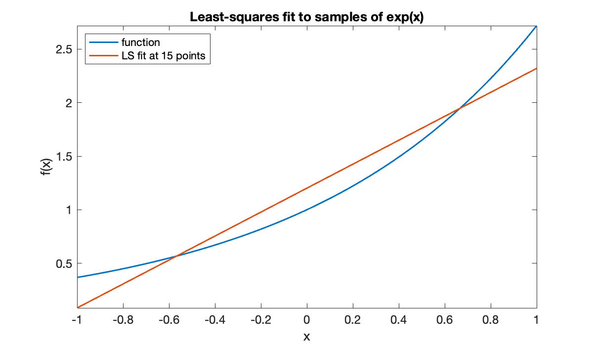

There’s nothing special about 15 points. Choosing more doesn’t change the result much.

t = linspace(-1, 1, 150)';
y = exp(t);
V = [t.^0, t];
c = V \ y;
p = @(t) c(1) + c(2)*t;
fplot(p, [-1, 1], displayname="LS fit at 150 points")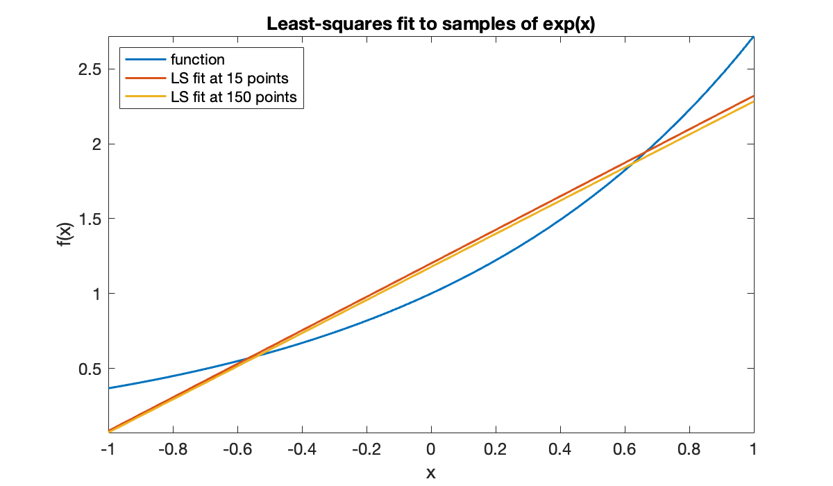

This situation is unlike interpolation, where the degree of the interpolant increases with the number of nodes. Here, the linear fit is apparently approaching a limit that we may think of as a continuous least-squares fit.

n = (40:60:400)';
slope = zeros(size(n));
intercept = zeros(size(n));

for k = 1:length(n)
    t = linspace(-1, 1, n(k))';
    V = [t.^0, t];
    c = V \ exp(t);
    intercept(k) = c(1);
    slope(k) = c(2);
end
disp(table(n, intercept, slope))

     n     intercept    slope

    ___    _________    ______

     40     1.1846      1.1091

    100     1.1789      1.1058

    160     1.1775       1.105

    220     1.1769      1.1046

    280     1.1765      1.1044

    340     1.1763      1.1043

    400     1.1761      1.1042

9.5 Trigonometric interpolation¶

Example 9.5.1

We will get a cardinal function without using an explicit formula, just by passing data that is 1 at one node and 0 at the others.

N = 7;  n = (N-1) / 2;
t = 2 * (-n:n)' / N;
y = zeros(N, 1);  y(n+1) = 1;
clf,  scatter(t, y, 'k'),  hold on

p = triginterp(t, y);
fplot(p, [-1, 1])
xlabel('x'),  ylabel('p(x)')   
title('Trig cardinal function')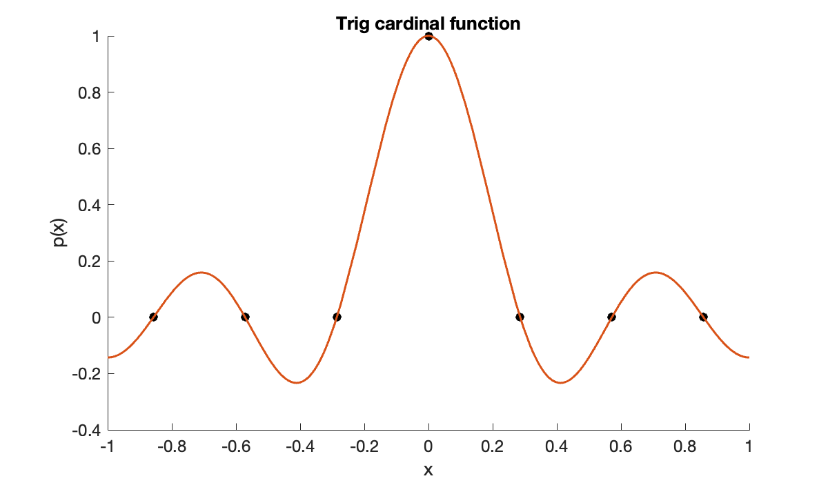

Here is a 2-periodic function and one of its interpolants.

clf
f = @(x) exp( sin(pi*x) - 2 * cos(pi*x) );
fplot(f, [-1, 1], displayname="periodic function"),  hold on
fplot(triginterp(t, f(t)), [-1, 1], displayname="trig interpolant")
y = f(t);  scatter(t, f(t), 'k')
xlabel('x'),  ylabel('f(x)')   
title('Trig interpolation');  legend()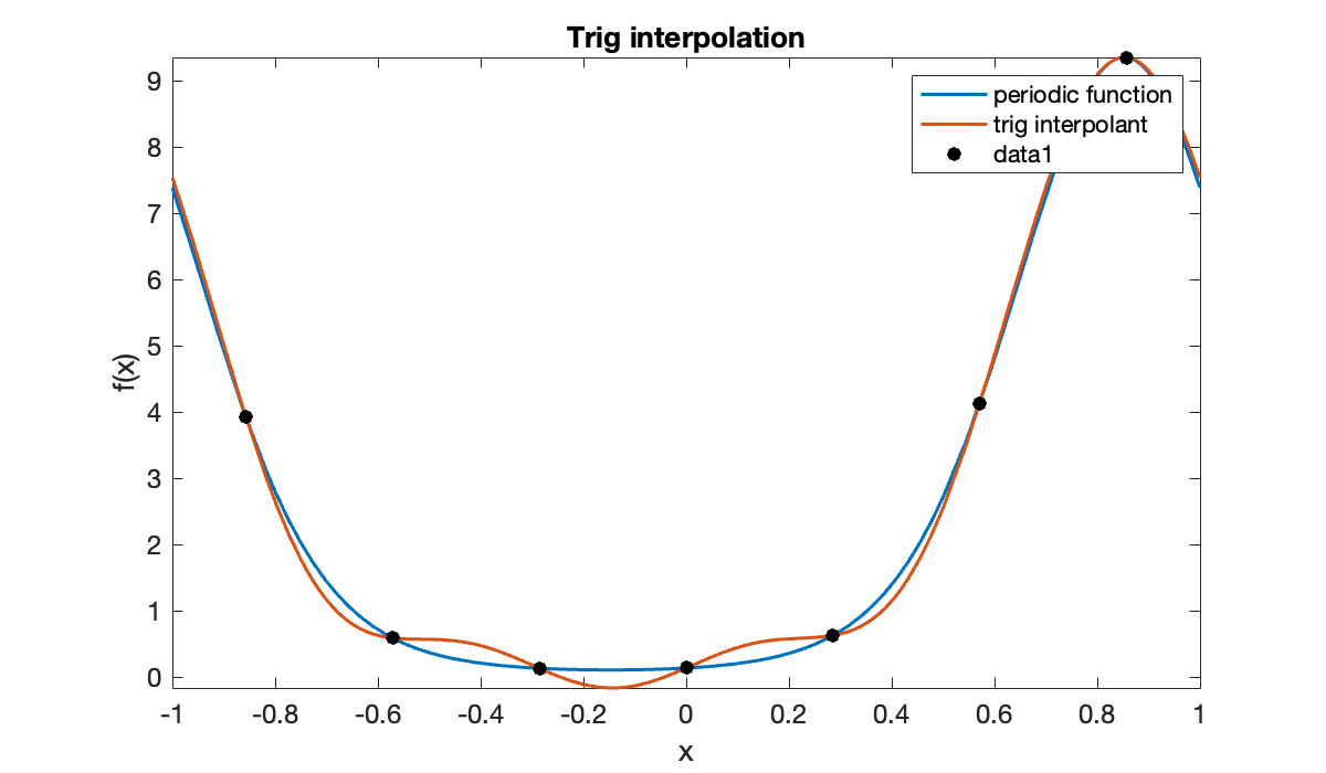

The convergence of the interpolant is spectral. We let $N$ go needlessly large here in order to demonstrate that unlike polynomials, trigonometric interpolation is stable on equally spaced nodes. Note that when $N$ is even, the value of $n$ is not an integer but works fine for defining the nodes.

N = 2:2:60;
err = zeros(size(N));
x = linspace(-1, 1, 1601)';  % for measuring error
for k = 1:length(N)
    n = (N(k) - 1) / 2;
    t = 2 * (-n:n)' / N(k);
    p = triginterp(t, f(t));
    err(k) = norm(f(x) - p(x), Inf);
end
clf,  semilogy(N, err, 'o-')
axis tight, title('Convergence of trig interpolation')   
xlabel('N'),  ylabel('max error')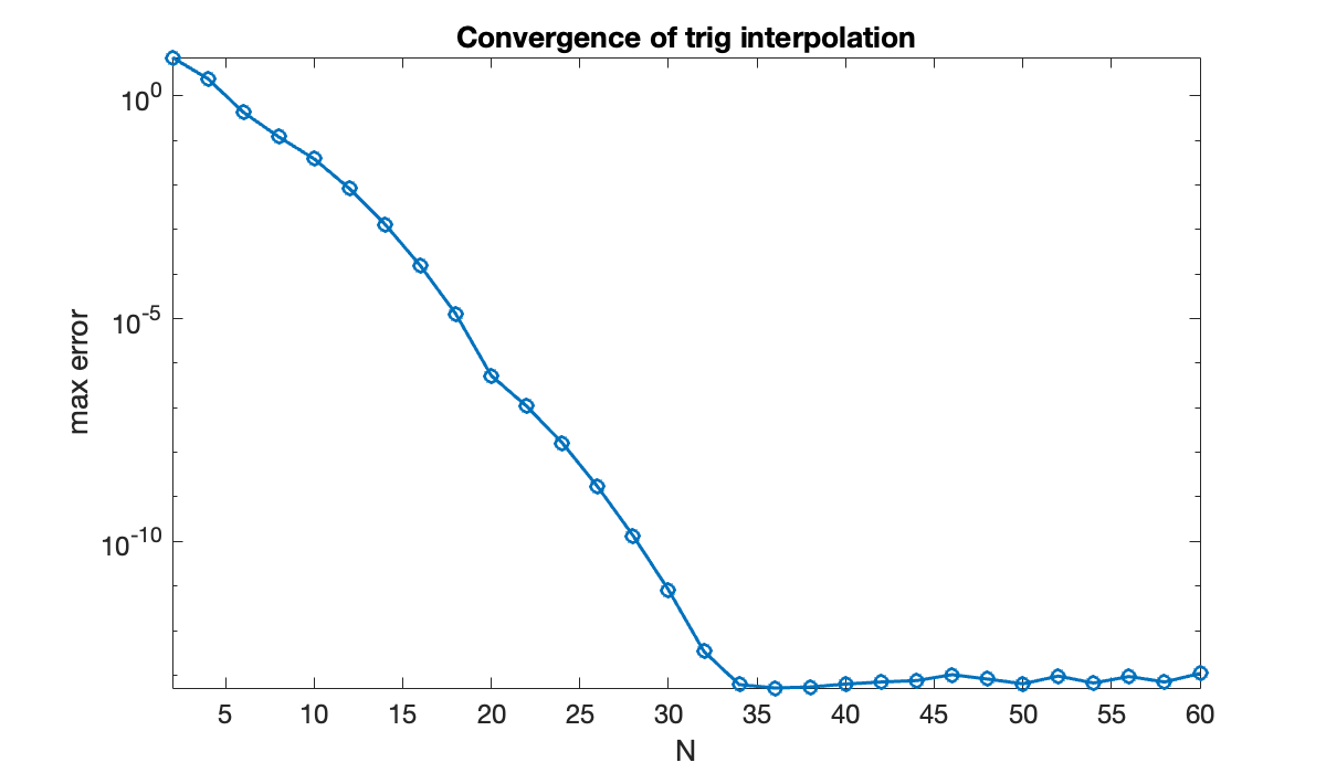

Example 9.5.2

This function has frequency content at $2\pi$ , $-2\pi$ , and π.

f = @(x) 3 * cos(2*pi * x) - exp(1i*pi * x);

To use fft, we set up nodes in the interval $[0,2)$ .

n = 4;
N = 2*n + 1;
t = 2 * (0:N-1)' / N;      % nodes in $[0,2)$
y = f(t);

We perform Fourier analysis using fft and then examine the resulting coefficients.

c = fft(y) / N;
freq = [0:n, -n:-1]';
format short
disp(table(freq, c, variableNames=["k", "coefficient"]))

    k           coefficient

    __    _______________________

     0    -7.4015e-17+0i

     1             -1+3.1961e-16i

     2            1.5-6.7735e-16i

     3     2.0068e-16-3.7007e-17i

     4     9.8686e-17+2.1124e-16i

    -4     9.6148e-17-2.5176e-16i

    -3     2.4341e-16-3.7007e-17i

    -2            1.5+7.2403e-16i

    -1    -9.6148e-17-2.5176e-16i

Note that $1.5 e^{2i\pi x}+1.5 e^{-2i\pi x} = 3 \cos(2\pi x)$ , so this result is sensible.

Fourier’s greatest contribution to mathematics was to point out that every periodic function is just a combination of frequencies—infinitely many of them in general, but truncated for computational use. Here we look at the magnitudes of the coefficients for $f(x) = \exp( \sin(\pi x) )$ .

f = @(x) exp( sin(pi*x) );    % content at all frequencies
n = 9;  N = 2*n + 1;
t = 2 * (0:N-1)' / N;         % nodes in $[0,2)$
y = f(t);
c = fft(y) / N;
freq = [0:n, -n:-1]';

clf
semilogy(freq, abs(c), 'o')
xlabel('k'),  ylabel('|c_k|')   
title('Fourier coefficients')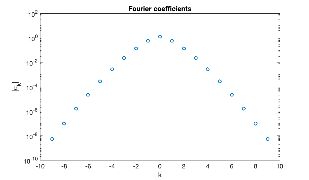

The Fourier coefficients of smooth functions decay exponentially in magnitude as a function of the frequency. This decay rate is determines the convergence of the interpolation error.

9.6 Spectrally accurate integration¶

Example 9.6.1

f = @(t) pi * sqrt( cos(pi*t).^2 + sin(pi*t).^2 / 4 );
N = (4:4:48)';
perim = zeros(size(N));
for k = 1:length(N)
    h = 2 / N(k);
    t = h * (0:N(k)-1);
    perim(k) = h * sum(f(t));
end
err = abs(perim - perim(end));    % use last value as "exact"
format long
disp(table(N, perim, err, variableNames=["number of nodes", "perimeter", "error"]))

    number of nodes       perimeter               error

    _______________    ________________    ____________________

           4           4.71238898038469       0.131835129889071

           8           4.83984155664137     0.00438255363239115

          12           4.84397070699574     0.00025340327802148

          16           4.84420619509697    1.79151767873975e-05

          20           4.84422270295636    1.40731740483346e-06

          24           4.84422399226142    1.18012335903472e-07

          28           4.84422409992693    1.03468327239398e-08

          32           4.84422410933683    9.36931421335885e-10

          36           4.84422411018687    8.68887184424239e-11

          40           4.84422411026561    8.14992517916835e-12

          44           4.84422411027305    7.14095449438901e-13

          48           4.84422411027376                       0

The approximations gain about one digit of accuracy for each constant increment of $n$ , which is consistent with spectral convergence.

Example 9.6.3

First consider the integral

\int_{-1}^1 \frac{1}{1+4x^2} \, dx = \arctan(2).

(1)

f = @(x) 1 ./ (1 + 4*x.^2);
exact = atan(2);

We compare the two spectral integration methods for a range of $n$ values.

n = (8:4:96)';
errCC = zeros(size(n));
errGL = zeros(size(n));
for k = 1:length(n)
  errCC(k) = exact - ccint(f, n(k));
  errGL(k) = exact - glint(f, n(k));
end
clf,  semilogy(n, abs([errCC errGL]), 'o-')
xlabel('number of nodes'),  ylabel('error')
title('Spectral integration')   
legend('Clenshaw–Curtis', 'Gauss–Legendre')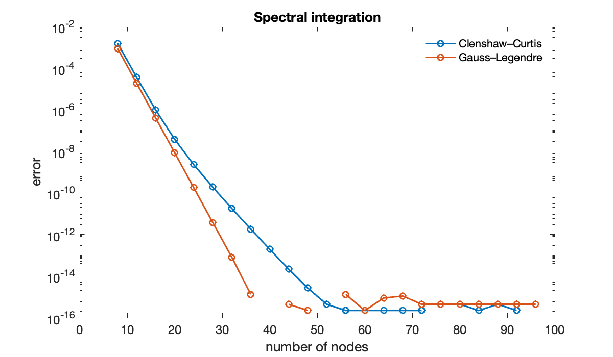

(The missing points are where the error is exactly zero.) Gauss–Legendre does converge faster here, but at something less than twice the rate.

Now we try a more sharply peaked integrand:

\int_{-1}^1 \frac{1}{1+16x^2} \, dx = \frac{1}{2}\arctan(4).

(2)

f = @(x) 1 ./ (1 + 16*x.^2);
exact = atan(4) / 2;

n = (8:4:96)';
errCC = zeros(size(n));
errGL = zeros(size(n));
for k = 1:length(n)
  errCC(k) = exact - ccint(f, n(k));
  errGL(k) = exact - glint(f, n(k));
end
clf,  semilogy(n, abs([errCC errGL]), 'o-')
xlabel('number of nodes'),  ylabel('error')
title('Spectral integration')   
legend('Clenshaw–Curtis', 'Gauss–Legendre')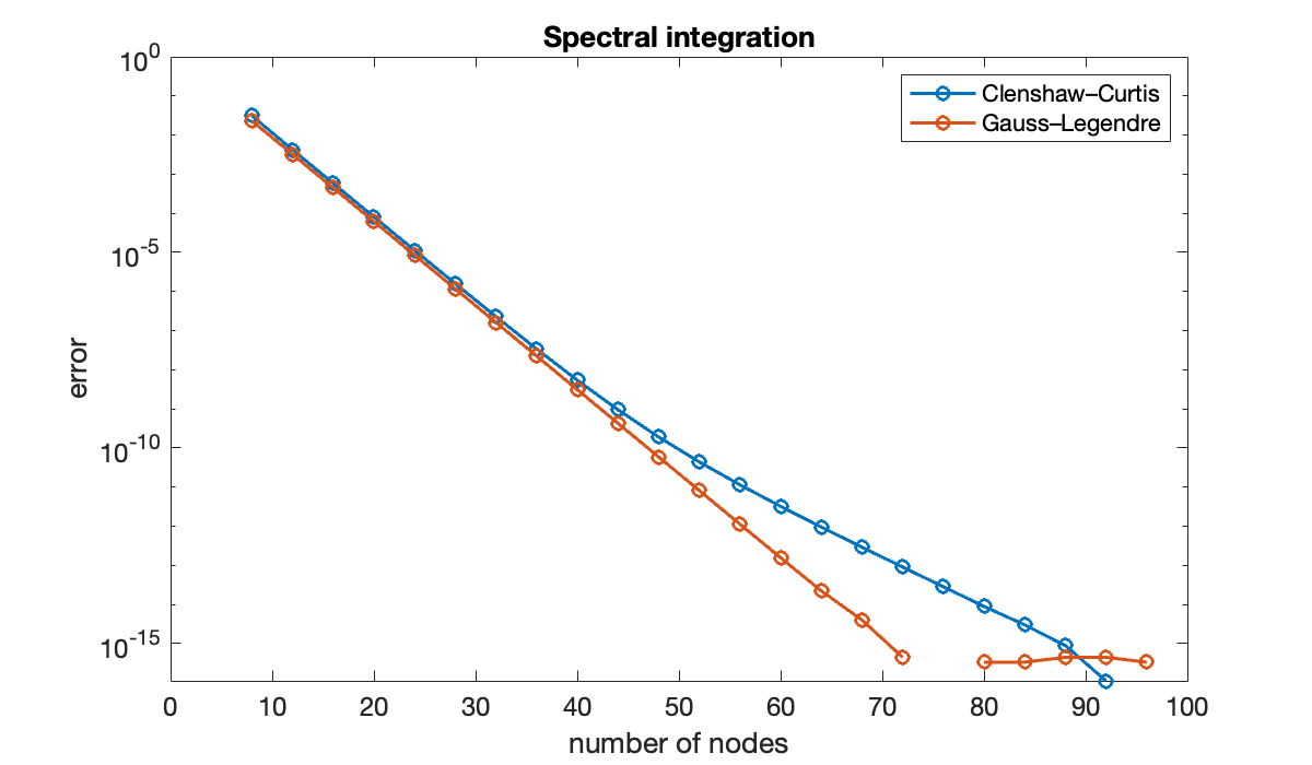

The two are very close until about $n=40$ , when the Clenshaw–Curtis method slows down.

Now let’s compare the spectral performance to that of our earlier adaptive method in intadapt. We will specify varying error tolerances and record the error as well as the total number of evaluations of $f$ .

tol = 10 .^ (-2:-2:-14)';
n = zeros(size(tol));  
errAdapt = zeros(size(tol));
for k = 1:length(n)
  [Q, t] = intadapt(f, -1, 1, tol(k));
  errAdapt(k) = exact - Q;
  n(k) = length(t);
end
hold on;  semilogy(n, abs(errAdapt), 'o-')
plot(n, n.^(-4), 'k--')        % 4th order error
set(gca, 'xscale', 'log')     
legend('ccint', 'glint', 'intadapt', '4th order')  
title(('Spectral vs 4th order'));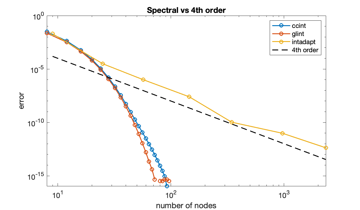

At the core of intadapt is a fourth-order formula, and the results track that rate closely. For all but the most relaxed error tolerances, both spectral methods are far more efficient than the low-order counterpart. For other integrands, particularly those that vary nonuniformly across the interval, the adaptive method might be more competitive.

9.7 Improper integrals¶

Example 9.7.2

f = @(x) 1 ./ (1 + x.^2);
clf,  subplot(2, 1, 1)
fplot(f, [-4, 4]);  set(gca, 'yscale', 'log') 
xlabel('x'),  ylabel('f(x)'),  ylim([1e-20, 1])  
title('Original integrand')   

x = @(t) sinh( pi * sinh(t) / 2 );
chain = @(t) pi/2 * cosh(t) .* cosh( pi * sinh(t) / 2 );
integrand = @(t) f(x(t)) .* chain(t);
subplot(2, 1, 2)
fplot(integrand, [-4, 4]);  set(gca, 'yscale', 'log') 
xlabel('t'), ylabel('f(x(t))'),  ylim([1e-20, 1])  
title('Transformed integrand')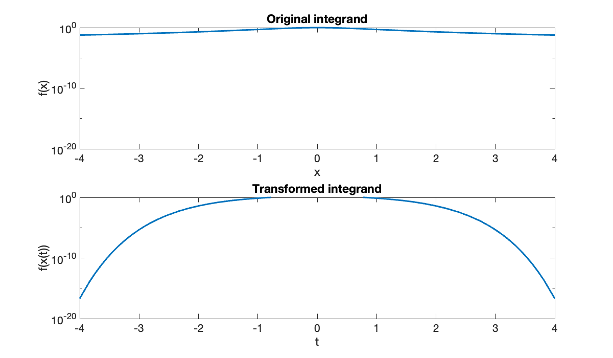

This graph suggests that we capture all of the integrand values that are larger than machine epsilon by integrating in $t$ from -4 to 4.

Example 9.7.3

f = @(x) 1 ./ (1 + x.^2);
tol = 1 ./ 10.^(5:0.5:14);
err = zeros(length(tol), 2);
len = zeros(length(tol), 2);
for k = 1:length(tol)
    [I1, x1] = intadapt(f, -2/tol(k), 2/tol(k), tol(k));
    [I2, x2] = intinf(f, tol(k));
    err(k, :) = abs(pi - [I1, I2]);
    len(k, :) = [length(x1), length(x2)];
end
clf,  loglog(len, err, 'o-')   
n = [100, 10000];
hold on,  loglog(n, 1000 * n.^(-4), 'k--')  % 4th order error
legend("direct", "double exponential", "4th order", location="southwest")
title(("Comparison of integration methods"));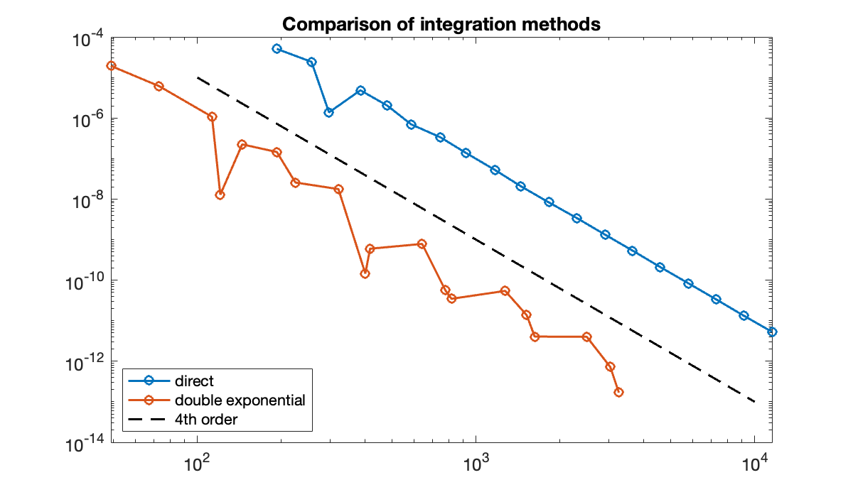

Both methods are roughly fourth-order due to Simpson’s formula in the underlying adaptive integration method. At equal numbers of evaluation nodes, however, the double exponential method is consistently 2–3 orders of magnitude more accurate.

Example 9.7.4

f = @(x) 1 ./ (10 * sqrt(x));
tol = 1 ./ 10.^(5:0.5:14);
err = zeros(length(tol), 2);
len = zeros(length(tol), 2);
for k = 1:length(tol)
    [I1, x1] = intadapt(f, (tol(k)/20)^2, 1, tol(k));
    [I2, x2] = intsing(f, tol(k));
    err(k, :) = abs(0.2 - [I1, I2]);
    len(k, :) = [length(x1), length(x2)];
end
clf,  loglog(len, err, 'o-')   
n = [30, 3000];
hold on,  loglog(n, 30 * n.^(-4), 'k--')  % 4th order error
legend("direct", "double exponential", "4th order", location="southwest")
title(("Comparison of integration methods"));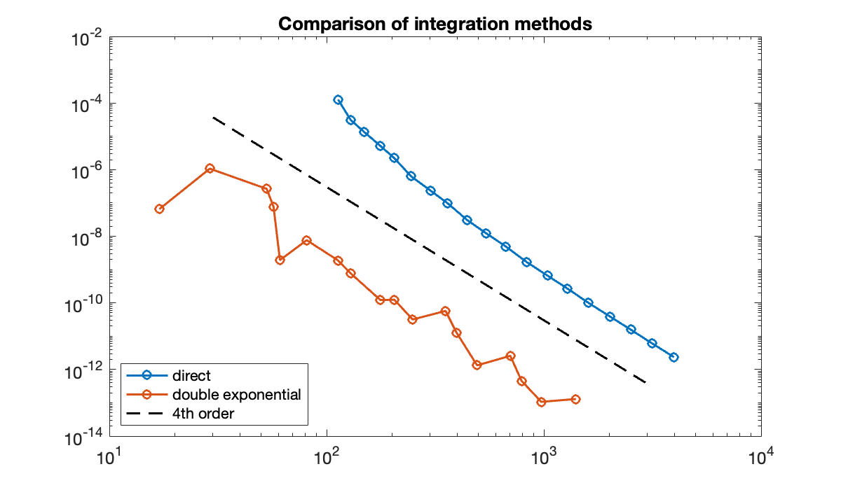

As in Demo 9.7.3, the double exponential method is more accurate than direct integration by a few orders of magnitude. Equivalently, the same accuracy can be reached with many fewer nodes.