Functions
Power iteration
1 2 3 4 5 6 7 8 9 10 11 12 13 14 15 16 17 18function [gamma,x] = poweriter(A,numiter) % POWERITER Power iteration for the dominant eigenvalue. % Input: % A square matrix % numiter number of iterations % Output: % gamma sequence of eigenvalue approximations (vector) % x final eigenvector approximation n = length(A); x = randn(n,1); x = x/norm(x,inf); for k = 1:numiter y = A*x; [normy,m] = max(abs(y)); gamma(k) = y(m)/x(m); x = y/y(m); end
Inverse iteration
1 2 3 4 5 6 7 8 9 10 11 12 13 14 15 16 17 18 19 20 21function [gamma,x] = inviter(A,s,numiter) % INVITER Shifted inverse iteration for the closest eigenvalue. % Input: % A square matrix % s value close to targeted eigenvalue (complex scalar) % numiter number of iterations % Output: % gamma sequence of eigenvalue approximations (vector) % x final eigenvector approximation n = length(A); x = randn(n,1); x = x/norm(x,inf); B = A - s*eye(n); [L,U] = lu(B); for k = 1:numiter y = U \ (L\x); [normy,m] = max(abs(y)); gamma(k) = x(m)/y(m) + s; x = y/y(m); end
Arnoldi iteration
1 2 3 4 5 6 7 8 9 10 11 12 13 14 15 16 17 18 19 20 21 22 23 24 25 26function [Q,H] = arnoldi(A,u,m) % ARNOLDI Arnoldi iteration for Krylov subspaces. % Input: % A square matrix (n by n) % u initial vector % m number of iterations % Output: % Q orthonormal basis of Krylov space (n by m+1) % H upper Hessenberg matrix, A*Q(:,1:m)=Q*H (m+1 by m) n = length(A); Q = zeros(n,m+1); H = zeros(m+1,m); Q(:,1) = u/norm(u); for j = 1:m % Find the new direction that extends the Krylov subspace. v = A*Q(:,j); % Remove the projections onto the previous vectors. for i = 1:j H(i,j) = Q(:,i)'*v; v = v - H(i,j)*Q(:,i); end % Normalize and store the new basis vector. H(j+1,j) = norm(v); Q(:,j+1) = v/H(j+1,j); end
GMRES
1 2 3 4 5 6 7 8 9 10 11 12 13 14 15 16 17 18 19 20 21 22 23 24 25 26 27 28 29 30 31 32 33 34 35 36function [x,residual] = arngmres(A,b,m) % ARNGMRES GMRES for a linear system (demo only). % Input: % A square matrix (n by n) % b right-hand side (n by 1) % M number of iterations % Output: % x approximate solution (n by 1) % r history of norms of the residuals n = length(A); Q = zeros(n,m+1); Q(:,1) = b/norm(b); H = zeros(m+1,m); % Initial "solution" is zero. residual(1) = norm(b); for j = 1:m % Next step of Arnoldi iteration. v = A*Q(:,j); for i = 1:j H(i,j) = Q(:,i)'*v; v = v - H(i,j)*Q(:,i); end H(j+1,j) = norm(v); Q(:,j+1) = v/H(j+1,j); % Solve the minimum residual problem. r = norm(b)*eye(j+1,1); z = H(1:j+1,1:j) \ r; x = Q(:,1:j)*z; residual(j+1) = norm( A*x - b ); end
Examples
8.1 Sparsity and structure
Example 8.1.1
Here we load the adjacency matrix of a graph with 2790 nodes. Each node is a web page referring to Roswell, NM, and the edges represent links between web pages. (Credit goes to Panayiotis Tsaparas and the University of Toronto for making this data public.)
load roswelladj
a = whos('A')We may define the density of as the number of nonzeros divided by the total number of entries.
Tip
Use nnz to count the number of nonzeros in a sparse matrix.
sz = size(A);  n = sz(1);
density = nnz(A) / prod(sz)The computer memory consumed by any variable can be discovered using whos. We can use it to compare the space needed for the sparse representation to its dense counterpart, that is, the space needed to store all the elements, whether zero or not.
F = full(A);
f = whos('F');
storage_ratio = f.bytes / a.bytesMatrix-vector products are also much faster using the sparse form because operations with structural zeros are skipped.
x = randn(n,1);
tic, for i = 1:200, A*x; end
sparse_time = toctic, for i = 1:200, F*x; end
dense_time = tocHowever, the sparse storage format in MATLAB is column-oriented. Operations on rows may take a lot longer than similar ones on columns.
v = A(:, 1000);
tic, for i = 1:n, A(:, i) = v; end
column_time = toc
r = v';
tic, for i = 1:n, A(i, :) = r; end
row_time = tocExample 8.1.2
Here is the adjacency matrix of a graph representing a small-world network, featuring connections to neighbors and a small number of distant contacts.
load smallworld.mat
G = graph(A);
plot(G, nodecolor='r')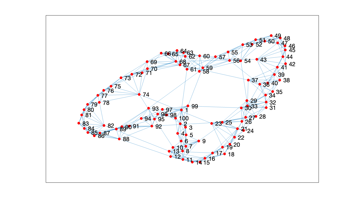
Because each node connects to relatively few others, the adjacency matrix is quite sparse.
spy(A)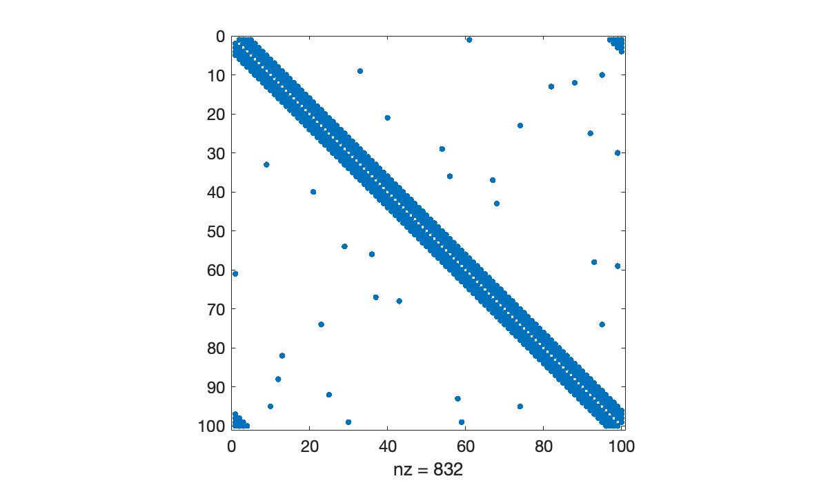
By Theorem 7.1.1, the entries of give the number of walks of length between pairs of nodes, as with “k degrees of separation” within a social network. As grows, the density of also grows.
clf
tiledlayout(2, 2)
for k = [2, 3, 4, 6]
    nexttile
    spy(A^k)
    title(sprintf("A^{%d}", k))
end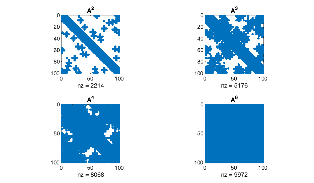
Example 8.1.3
The spdiags function creates a sparse matrix given its diagonal elements. The main or central diagonal is numbered zero, above and to the right of that is positive, and below and to the left is negative.
n = 50;
n = 50;
% Put constant values on 3 diagonals
A = spdiags([n, 1, 0.1], [-3, 0, 5], n, n);
% Put other values on 1st superdiagonal
A = spdiags(-(0:n-1)', 1, A);
full(A(1:7, 1:7))Without pivoting, the LU factors have the same lower and upper bandwidth as the original matrix.
Tip
The sparse function converts any matrix to sparse form. But it’s usually better to construct a sparse matrix directly, as the standard form might not fit in memory.
[L, U] = lufact(A);
clf
subplot(1, 2, 1), spy(L), title('L')
subplot(1, 2, 2), spy(U), title(('U'));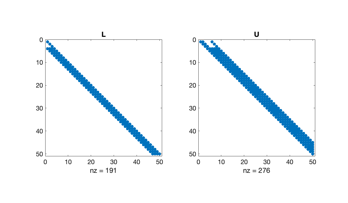
However, if we introduce row pivoting, bandedness may be expanded or destroyed.
[L, U, p] = plufact(A);
subplot(1, 2, 1), spy(L(p, :)), title('L')
subplot(1, 2, 2), spy(U), title(('U'));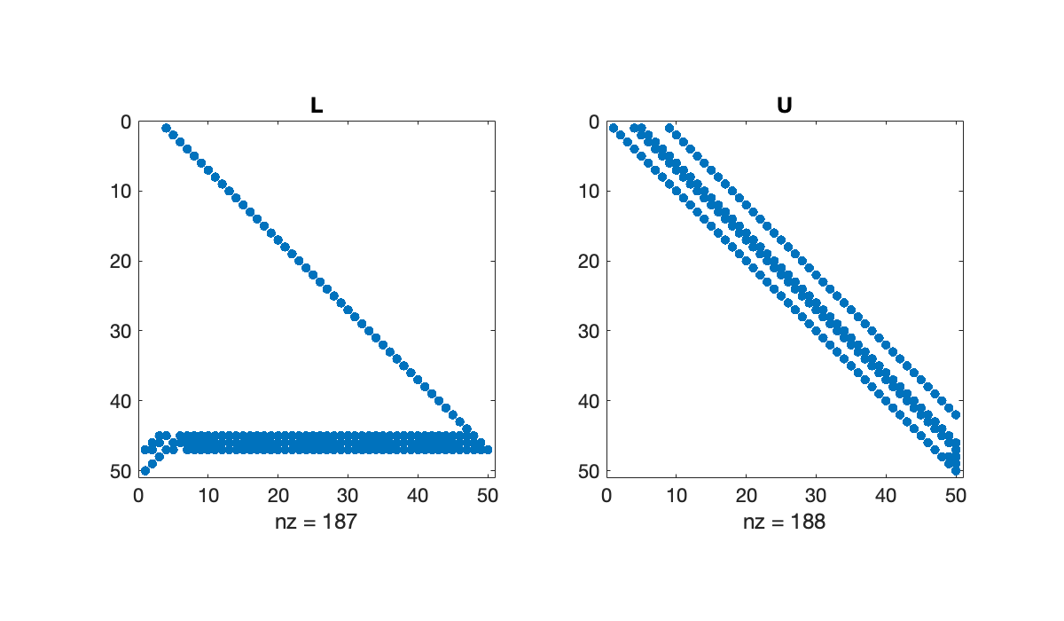
Example 8.1.4
The following generates a random sparse matrix with prescribed eigenvalues.
n = 4000;
density = 4e-4;
lambda = 1 ./ (1:n);
A = sprandsym(n, density, lambda);
clf,  spy(A)
title('Sparse symmetric matrix')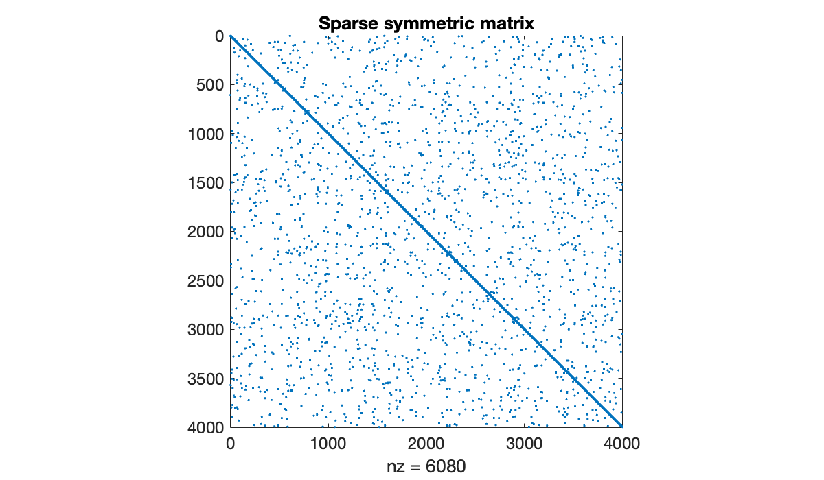
The eigs function finds a small number eigenvalues meeting some criterion. First, we ask for the 5 of largest (complex) magnitude.
[V, D] = eigs(A, 5);    % largest magnitude
1 ./ diag(D) % should be 1, 2, 3, 4, 5Now we find the 4 closest to the value 0.03 in the complex plane.
[V, D] = eigs(A, 4, 0.03);    % closest to 0.03
diag(D)The time needed to solve a sparse linear system is not easy to predict unless you have some more information about the matrix. But it will typically be orders of magnitude faster than the dense version of the same problem.
x = 1 ./ (1:n)';
b = A * x;
tic, sparse_err = norm(x - A\b), sparse_time = tocF = full(A);
tic, dense_err = norm(x - F\b), dense_time = toc8.2 Power iteration
Example 8.2.1
Here we choose a magic 5×5 matrix and a random 5-vector.
A = magic(5) / 65;
x = randn(5, 1);
Applying matrix-vector multiplication once doesn’t do anything recognizable.
y = A * xRepeating the multiplication still doesn’t do anything obvious.
z = A * yBut if we keep repeating the matrix-vector multiplication, something remarkable happens: .
for j = 1:8
    x = A * x;
end
[x, A * x]This phenomenon seems to occur regardless of the starting vector.
x = randn(5, 1);
for j = 1:8
    x = A * x;
end
[x, A * x]Example 8.2.2
We will experiment with the power iteration on a 5×5 matrix with prescribed eigenvalues and dominant eigenvalue at 1.
ev = [1, -0.75, 0.6, -0.4, 0];
% Make a triangular matrix with eigenvalues on the diagonal.
A = triu(ones(5, 5), 1) + diag(ev);
We run the power iteration 60 times. The best estimate of the dominant eigenvalue is the last entry of the first output.
[beta, x] = poweriter(A, 60);
format long
beta(1:12)We check for linear convergence using a log-linear plot of the error.
err = 1 - beta;
clf,  semilogy(abs(err), '.-')
title('Convergence of power iteration')
xlabel('k'),  ylabel(('|\lambda_1 - \beta_k|'));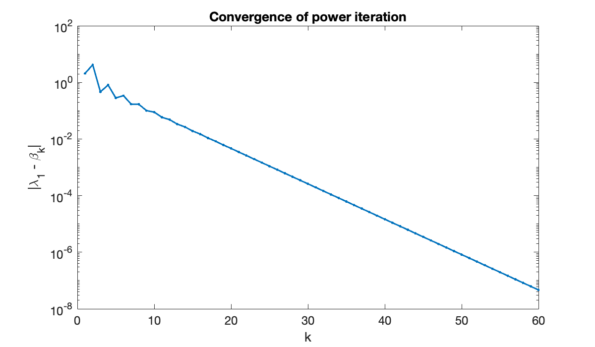
The asymptotic trend seems to be a straight line, consistent with linear convergence. To estimate the convergence rate, we look at the ratio of two consecutive errors in the linear part of the convergence curve. The ratio of the first two eigenvalues should match the observed rate.
theory = ev(2) / ev(1)
observed = err(40) / err(39)Note that the error is supposed to change sign on each iteration. The effect of these alternating signs is that estimates oscillate around the exact value.
beta(26:29)In practical situations, we don’t know the exact eigenvalue that the algorithm is supposed to find. In that case we would base errors on the final β that was found, as in the following plot.
err = beta(end) - beta(1:end-1);
semilogy(abs(err), '.-')
title('Convergence of power iteration')
xlabel('k'),  ylabel(('|\beta_{60} - \beta_k|'));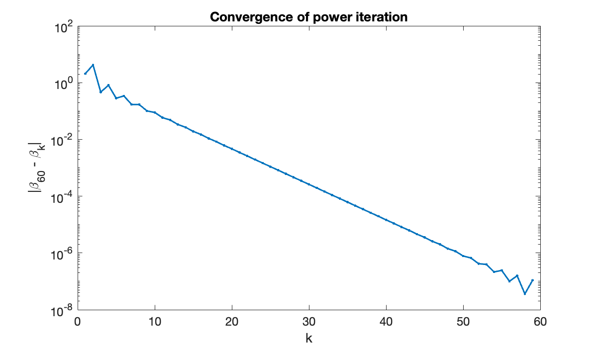
The results are very similar until the last few iterations, when the limited accuracy of the reference value begins to show. That is, while it is a good estimate of , it is less good as an estimate of the error in nearby estimates.
8.3 Inverse iteration
Example 8.3.1
We set up a triangular matrix with prescribed eigenvalues on its diagonal.
ev = [1, -0.75, 0.6, -0.4, 0];
A = triu(ones(5, 5), 1) + diag(ev);
We run inverse iteration with the shift . The result should converge to the eigenvalue closest to 0.7, which we know to be 0.6 here.
s = 0.7;
[beta, x] = inviter(A, s, 30);
format short
beta(1:10)The convergence is again linear.
err = abs(0.6 - beta);
semilogy(abs(err),'.-')
title('Convergence of inverse iteration')
xlabel('k'), ylabel(('|\lambda_j - \beta_k|'));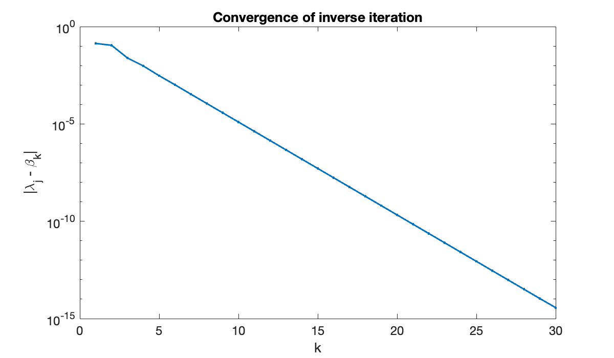
Let’s reorder the eigenvalues to enforce (8.3.3).
Tip
The second output of sort returns the index permutation needed to sort the given vector.
[~, idx] = sort(abs(ev - s));
ev = ev(idx)Now it is easy to compare the theoretical and observed linear convergence rates.
theoretical_rate = (ev(1) - s) / (ev(2) - s)
observed_rate = err(26) / err(25)Example 8.3.2
ev = [1, -0.75, 0.6, -0.4, 0];
A = triu(ones(5, 5), 1) + diag(ev);
We begin with a shift , which is closest to the eigenvalue 0.6.
s = 0.7;
x = ones(5, 1);
y = (A - s * eye(5)) \ x;
beta = x(1) / y(1) + sNote that the result is not yet any closer to the targeted 0.6. But we proceed (without being too picky about normalization here).
s = beta;
x = y / y(1);
y = (A - s * eye(5)) \ x;
beta = x(1) / y(1) + sStill not much apparent progress. However, in just a few more iterations the results are dramatically better.
format long
for k = 1:4
    s = beta;
    x = y / y(1);
    y = (A - s * eye(5)) \ x;
    beta = x(1) / y(1) + s
end8.4 Krylov subspaces
Example 8.4.1
First we define a triangular matrix with known eigenvalues, and a random vector .
lambda = 10 + (1:100);
A = diag(lambda) + triu(rand(100), 1);
b = rand(100, 1);
Next we build up the first ten Krylov matrices iteratively, using renormalization after each matrix-vector multiplication.
Km = b;
for m = 1:29
    v = A * Km(:, m);
    Km(:, m+1) = v / norm(v);
end
Now we solve least-squares problems for Krylov matrices of increasing dimension, recording the residual in each case.
warning off
resid = zeros(30, 1);
for m = 1:30
    z = (A * Km(:, 1:m)) \ b;
    x = Km(:, 1:m) * z;
    resid(m) = norm(b - A * x);
end
The linear system approximations show smooth linear convergence at first, but the convergence stagnates after only a few digits have been found.
clf
semilogy(resid, '.-')
xlabel('m'),  ylabel('|| b-Ax_m ||')
set(gca,'ytick',10.^(-6:2:0))
axis tight, title('Residual for linear systems')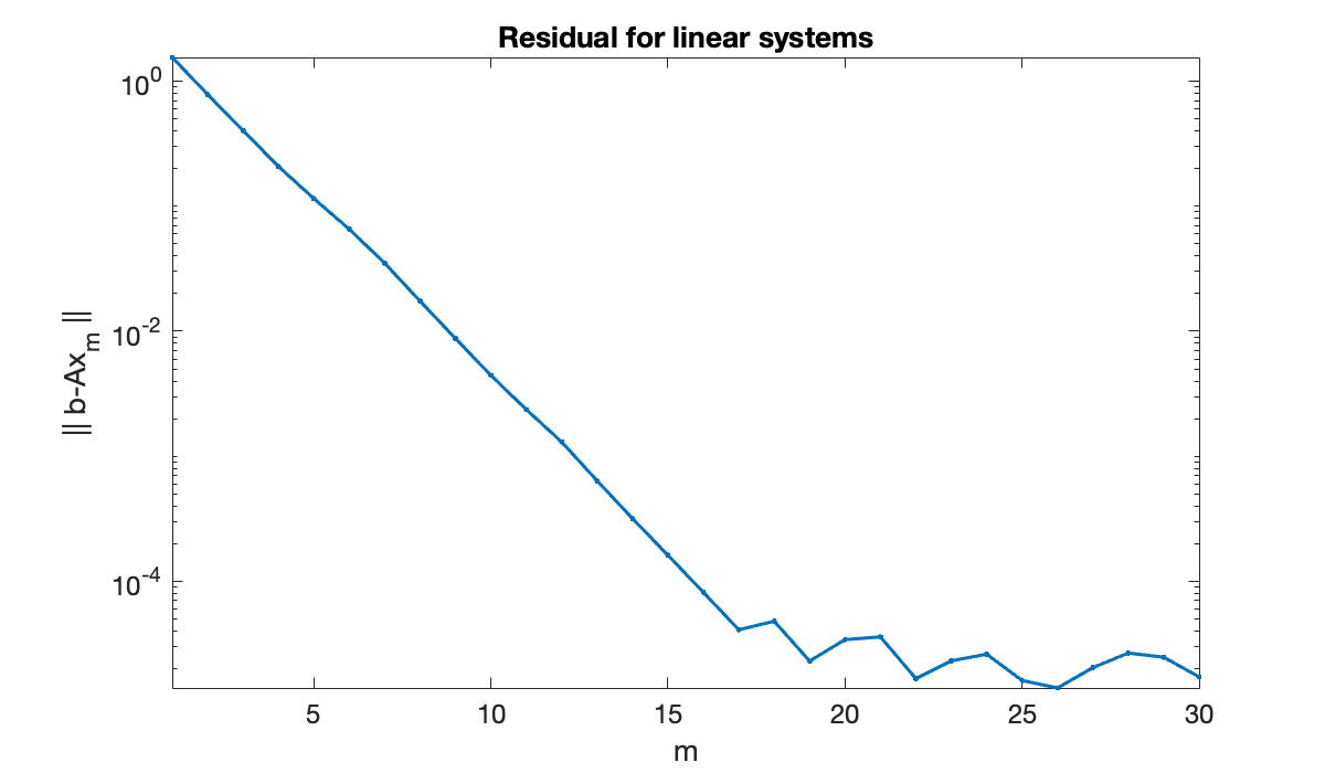
Example 8.4.2
We illustrate a few steps of the Arnoldi iteration for a small matrix.
A = randi(9, [6, 6])The seed vector we choose here determines the first member of the orthonormal basis.
u = randn(6, 1);
Q = u / norm(u);
Multiplication by gives us a new vector in .
Aq = A * Q(:, 1);We subtract off its projection in the previous direction. The remainder is rescaled to give us the next orthonormal column.
v = Aq - dot(Q(:, 1), Aq) * Q(:, 1);
Q = [Q, v / norm(v)];
On the next pass, we have to subtract off the projections in two previous directions.
Aq = A * Q(:, 2);
v = Aq - dot(Q(:, 1), Aq) * Q(:, 1) - dot(Q(:, 2), Aq) * Q(:, 2);
Q = [Q, v / norm(v)];
At every step, is an ONC matrix.
format
norm(Q' * Q - eye(3))And spans the same space as the three-dimensional Krylov matrix.
K = [u, A * u, A * A * u];
rank([Q, K])8.5 GMRES
Example 8.5.1
We define a triangular matrix with known eigenvalues and a random vector .
lambda = 10 + (1:100);
A = diag(lambda) + triu(rand(100), 1);
b = rand(100, 1);
Instead of building the Krylov matrices, we use the Arnoldi iteration to generate equivalent orthonormal vectors.
[Q, H] = arnoldi(A, b, 60);The Arnoldi bases are used to solve the least-squares problems defining the GMRES iterates.
resid = norm(b);
for m = 1:60
    s = [norm(b); zeros(m, 1)];
    z = H(1:m+1, 1:m) \ s;
    x = Q(:, 1:m) * z;
    resid = [resid, norm(b - A * x)];
end
The approximations converge smoothly, practically all the way to machine epsilon.
clf
semilogy(resid,'.-')
xlabel('m'),  ylabel('|| b - Ax_m ||')
axis tight, title(('Residual for GMRES'));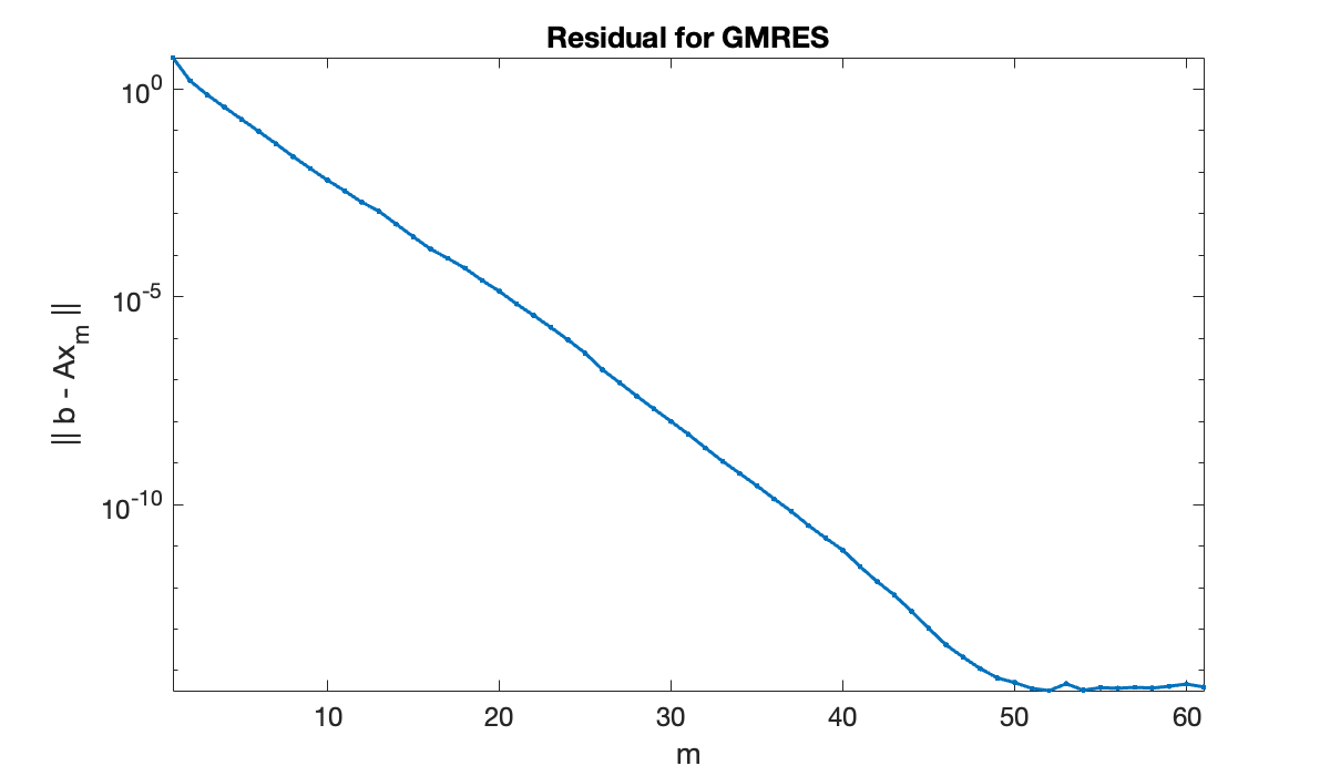
Example 8.5.2
The following experiments are based on a matrix resulting from discretization of a partial differential equation.
d = 50;
A = d^2 * gallery('poisson', d);
n = size(A, 1)
b = ones(n, 1);
clf, spy(A)We compare unrestarted GMRES with three different thresholds for restarting. Here we are using the built-in gmres, since our simple implementation does not offer restarting.
clf
restart = [120, 20, 40, 60];
for j = 1:4
    [~,~,~,~,rv] = gmres(A, b, restart(j), 1e-9,120 / restart(j));
    semilogy(0:length(rv) - 1, rv),  hold on
end
title('Convergence of restarted GMRES')
xlabel('m'),  ylabel('residual norm')
legend('no restart','every 20','every 40','every 60','location','southwest');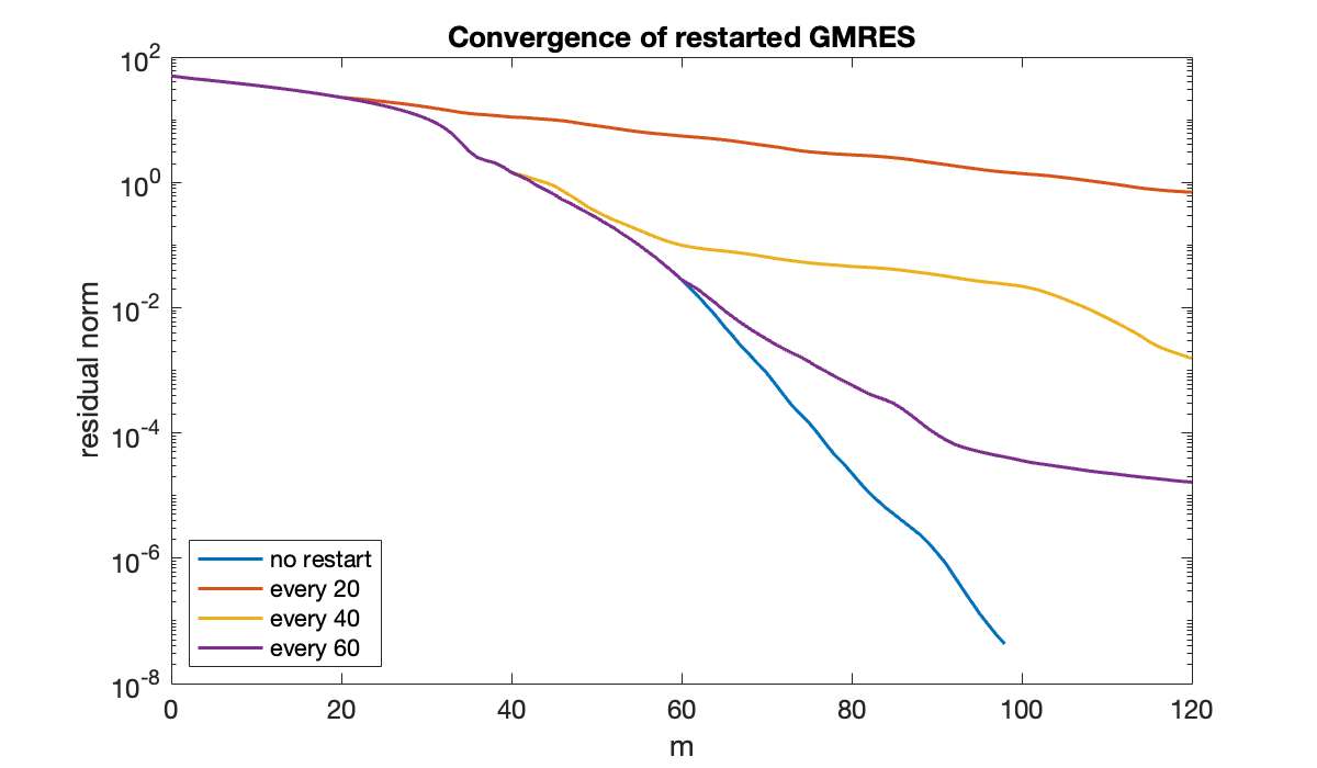
The “pure” GMRES curve is the lowest one. All of the other curves agree with it until the first restart. Decreasing the restart value makes the convergence per iteration generally worse, but the time required per iteration smaller as well.
8.6 MINRES and conjugate gradients
Example 8.6.2
The following matrix is indefinite.
A = (11 / pi)^2 * gallery('poisson', 10);
A = A - 20 * eye(100);
lambda = eig(full(A));
isneg = lambda < 0;
disp(sprintf("%d negative and %d positive eigenvalues", sum(isneg), sum(~isneg)))
13 negative and 87 positive eigenvalues
We can compute the relevant quantities from Theorem 8.6.1.
m = min(-lambda(isneg));
M = max(-lambda(isneg));
kappa_minus = M / m;
m = min(lambda(~isneg));
M = max(lambda(~isneg));
kappa_plus = M / m;
S = sqrt(kappa_minus * kappa_plus);
rho = sqrt((S - 1) / (S + 1));
fprintf("convergence rate: %.3f", rho)
convergence rate: 0.950Because the iteration number is halved in (8.6.4), the rate constant of linear convergence is the square root of this number, which makes it even closer to 1.
Now we apply MINRES to a linear system with this matrix, and compare the observed convergence to the upper bound from the theorem.
b = rand(100, 1);
[xMR, ~,~ , ~, residMR] = minres(A, b, 1e-10, 100);
relres = residMR / norm(b);
m = 0:length(relres) - 1;
clf,  semilogy(m, relres, '.-')
hold on
semilogy(m, rho .^ m, 'k--')
xlabel('m'),  ylabel('relative residual')
title('Convergence of MINRES')
legend('MINRES', 'upper bound', 'location', 'southwest');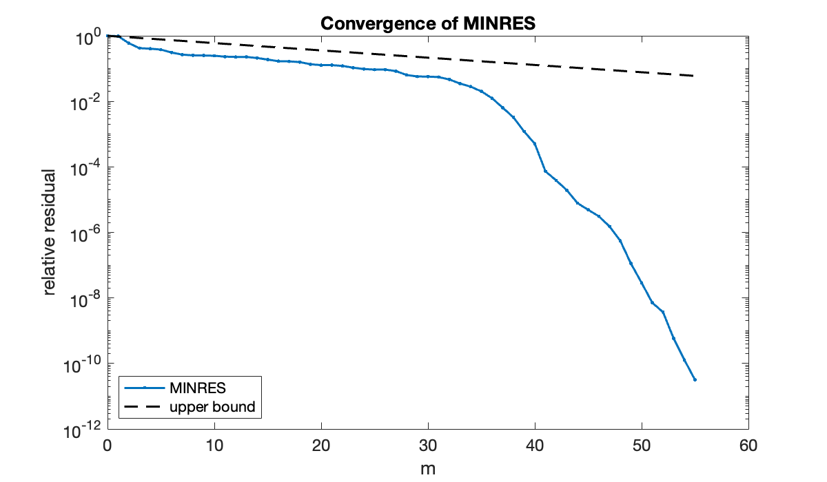
The upper bound turns out to be pessimistic here, especially in the later iterations. However, you can see a slow linear phase in the convergence that tracks the bound closely.
Example 8.6.3
We will compare MINRES and CG on some quasi-random SPD problems. The first matrix has a condition number of 100.
n = 5000;
density = 0.001;
A = sprandsym(n, density, 1e-2, 2);
We generate a system with a known solution.
x = (1:n)' / n;
b = A * x;
Now we apply both methods and compare the convergence of the system residuals.
[xMR, ~, ~, ~, residMR] = minres(A, b, 1e-7, 100);
[xCG, ~, ~, ~, residCG] = pcg(A, b, 1e-7, 100);
M = length(residMR) - 1;
clf,  semilogy(0:M, residMR / norm(b), '.-')
M = length(residCG) - 1;
hold on,  semilogy(0:M, residCG / norm(b), '.-')
title('Convergence of MINRES and CG')
xlabel('Krylov dimension m')
ylabel('||r_m|| / ||b||')
legend('MINRES', 'CG');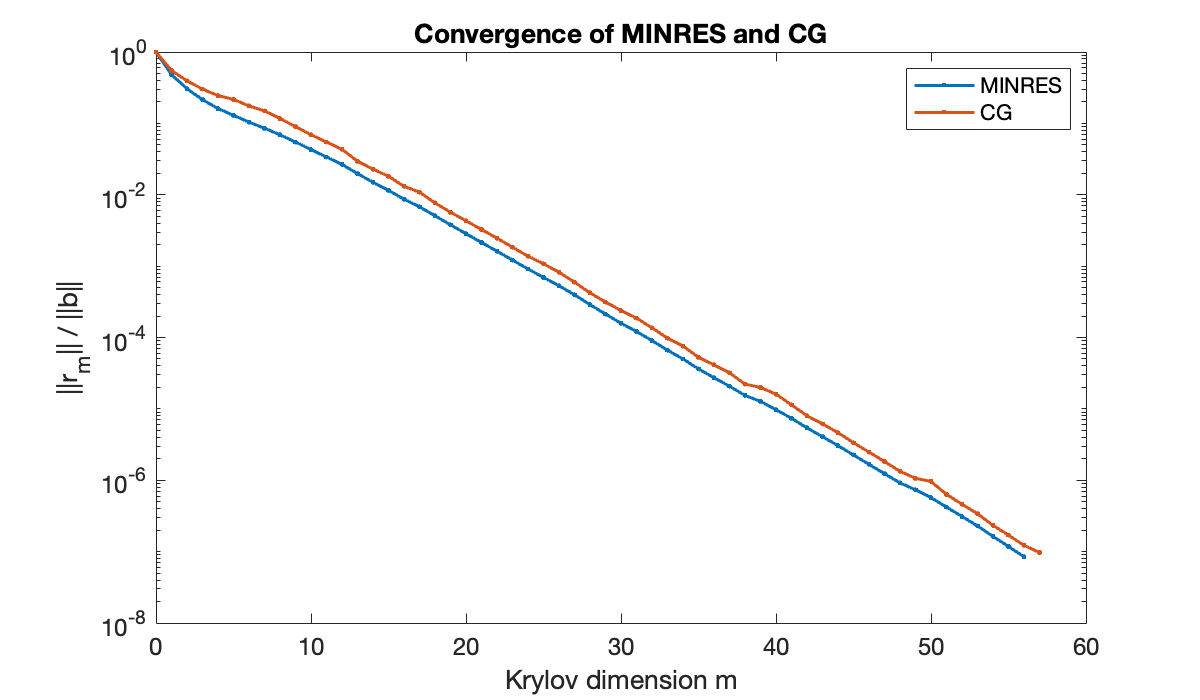
There is little difference between the two methods here. Next, we increase the condition number of the matrix by a factor of 25. The rule of thumb predicts that the number of iterations required should increase by a factor of about 5.
A = sprandsym(n, density, 1e-2 / 25, 2);
b = A * x;
[xMR, ~, ~, ~, residMR] = minres(A, b, 1e-7, 400);
[xCG, ~, ~, ~, residCG] = pcg(A, b, 1e-7, 400);
M = length(residMR) - 1;
clf, semilogy(0:M, residMR / norm(b), '.-')
M = length(residCG) - 1;
hold on, semilogy(0:M, residCG / norm(b), '.-')
title('Convergence of MINRES and CG')
xlabel('Krylov dimension m')
ylabel('||r_m|| / ||b||')
legend('MINRES', 'CG');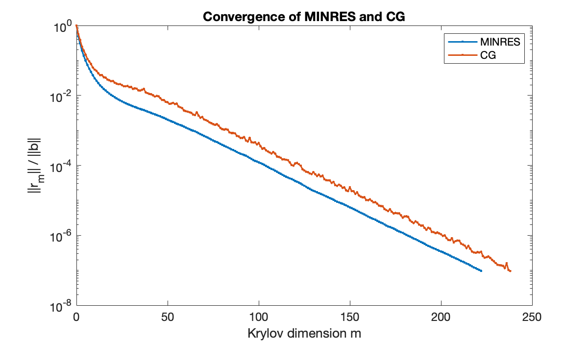
Both methods have an early superlinear phase that allow them to finish slightly sooner than the factor of 5 predicted: Theorem 8.6.2 is an upper bound, not necessarily an approximation. Both methods ultimately achieve the same reduction in the residual; MINRES stops earlier, but with a slightly larger error.
8.7 Matrix-free iterations
Example 8.7.1
We use a readily available test image.
load mandrill
[m, n] = size(X);
clf
imshow(X, [0, 255])
title('Original image')    % ignore this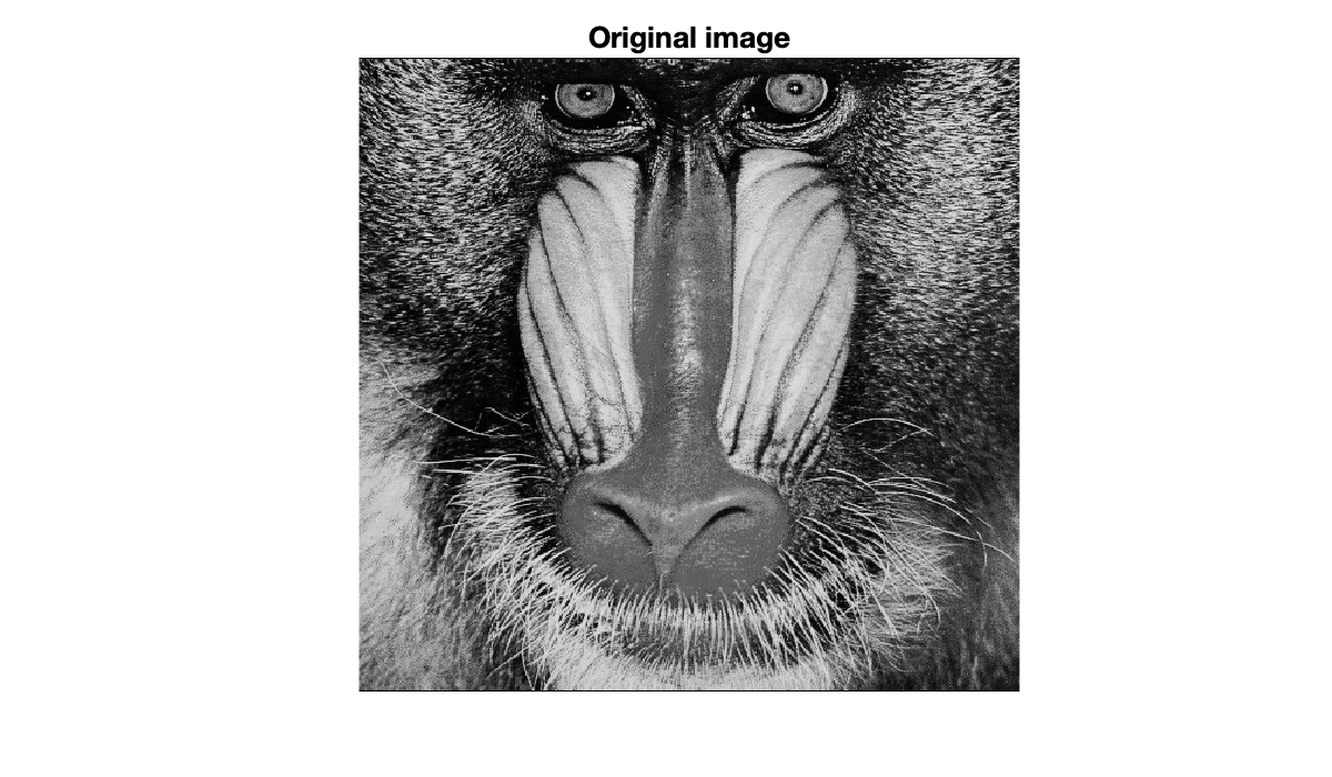
We define the one-dimensional tridiagonal blurring matrices.
v = [1/4, 1/2, 1/4];
B = spdiags(v, -1:1, m, m);
C = spdiags(v, -1:1, n, n);
Finally, we show the results of using repetitions of the blur in each direction.
blur = @(X) B^12 * X * C^12;
imshow(blur(X), [0, 255])
title(('Blurred image'));
Example 8.7.2
We repeat the earlier process to blur an original image to get .
load mandrill
[m, n] = size(X);
v = [1/4, 1/2, 1/4];
B = spdiags(v, -1:1, m, m);
C = spdiags(v, -1:1, n, n);
blur = @(X) B^12 * X * C^12;
Z = blur(X);
clf, imshow(Z, [0, 255])
title(("Blurred image"));
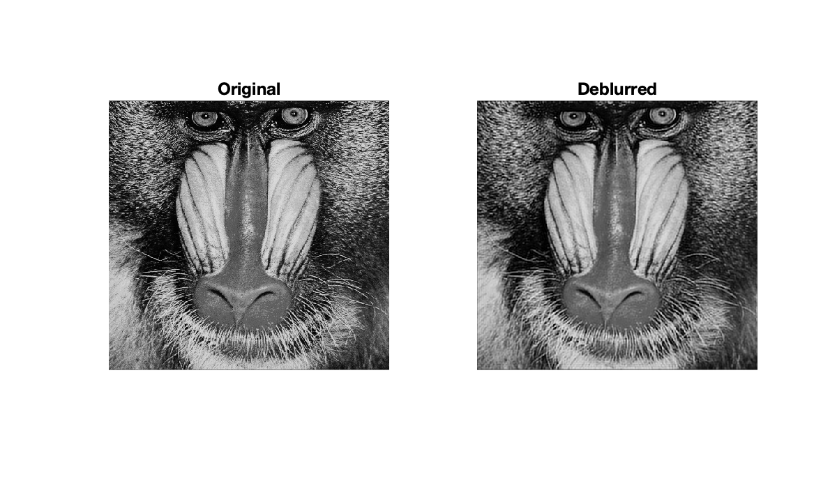
Now we imagine that is unknown and that we want to recover it from . We first need functions that translate between vector and matrix representations.
vec = @(X) reshape(X,m*n,1);
unvec = @(x) reshape(x,m,n);
T = @(x) vec( blur(unvec(x)) );
The blurring operators are symmetric, so we apply minres to the composite blurring transformation T.
y = gmres(T, vec(Z), 50, 1e-5);
Y = unvec(y);

subplot(121)
imshow(X, [0, 255])
title("Original")
subplot(122)
imshow(Y, [0, 255])
title(("Deblurred"));
gmres(50) converged at outer iteration 2 (inner iteration 45) to a solution with relative residual 1e-05.
8.8 Preconditioning
Example 8.8.1
Here is an SPD matrix that arises from solving partial differential equations.
A = gallery("wathen", 60, 60);
n = size(A, 1);
clf,  spy(A)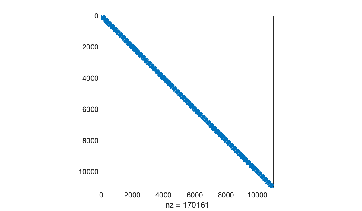
There is an easy way to use the diagonal elements of , or any other vector, as a diagonal preconditioner.
M = spdiags(diag(A), 0, n, n);We now compare MINRES with and without the preconditioner.
b = ones(n, 1);
[x, ~, ~, ~, resid_plain] = minres(A, b, 1e-10, 400);
clf,  semilogy(resid_plain)
xlabel('iteration number'), ylabel('residual norm')
title('Unpreconditioned MINRES')

[x, ~, ~, ~, resid_prec] = minres(A, b, 1e-10, 400, M);
hold on,  semilogy(resid_prec)
title('Precondtioned MINRES')
legend('no prec.', 'with prec.');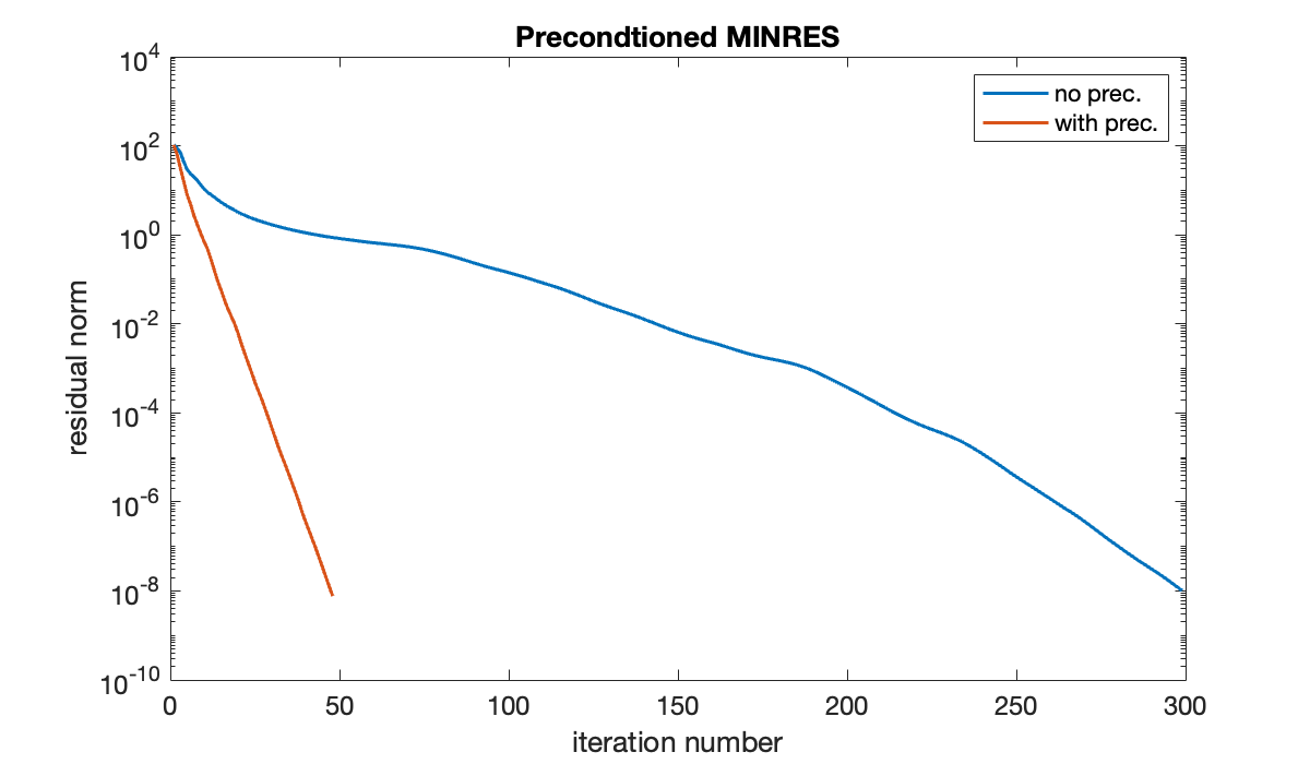
The diagonal preconditioner cut down substantially on the number of iterations. The effect on the total time is less dramatic, but this is not a large version of the problem.
Example 8.8.2
Here is a random nonsymmetric matrix.
n = 8000;
A = speye(n) + sprand(n, n, 0.00035);
Without a preconditioner, restarted GMRES makes slow progress.
b = rand(n, 1);
[x, ~, ~, ~, resid_plain] = gmres(A, b, 50, 1e-10, 3);  % restart at 50
format short e
resid_plain(1:30:end)This version of incomplete LU factorization simply prohibits fill-in for the factors, freezing the sparsity pattern of the approximate factors to match the original matrix.
[L, U] = ilu(A);
clf
subplot(121), spy(L)
title('L')
subplot(122), spy(U)
title('U')
disp(sprintf("There are %d nonzeros in A", nnz(A)))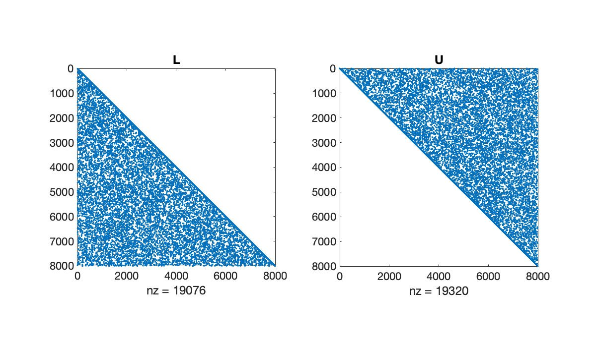
There are 30396 nonzeros in A
It does not produce a true factorization of .
norm( full(A - L * U) )The actual preconditioning matrix is . However, the gmres function allows setting the preconditioner by giving the factors independently.
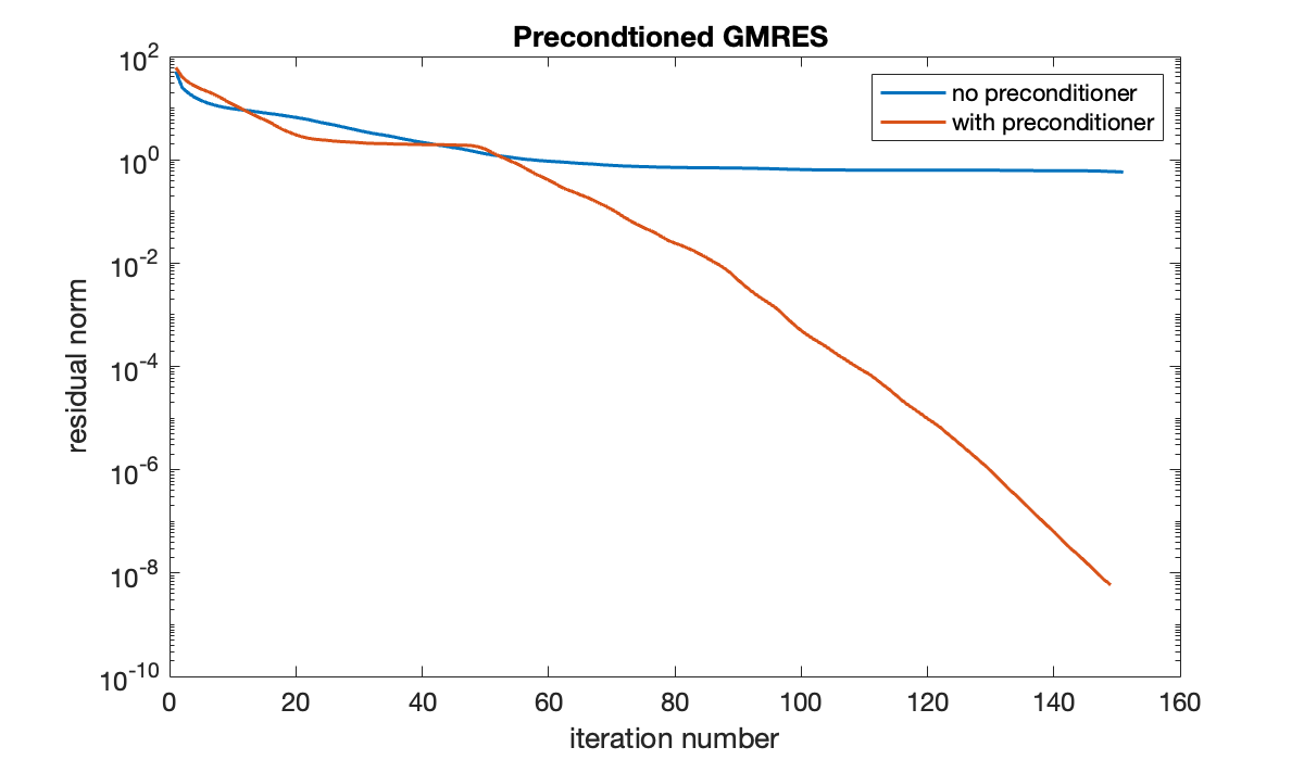
[x, ~, ~, ~, resid_prec] = gmres(A, b, [], 1e-10, 300, L, U);The preconditioner makes a significant difference in the number of iterations needed.
clf, semilogy(resid_plain)
hold on, semilogy(resid_prec)
xlabel('iteration number'), ylabel('residual norm')
title('Precondtioned GMRES ')
legend('no preconditioner', 'with preconditioner');