Examples
7.1 From matrix to insight
Example 7.1.4
Here we create an adjacency matrix for a graph on four nodes.
A = [0 1 0 0; 1 0 0 0; 1 1 0 1; 0 1 1 0]Since this adjacency matrix is not symmetric, the edges are all directed. We use digraph to create a directed graph.
G = digraph(A);
plot(G)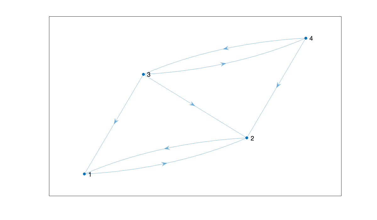
Here are the counts of all walks of length 3 in the graph:
A^3If the adjacency matrix is symmetric, the result is an undirected graph: all edges connect in both directions.
A = [0 1 1 0; 1 0 0 1; 1 0 0 0; 0 1 0 0];
plot(graph(A))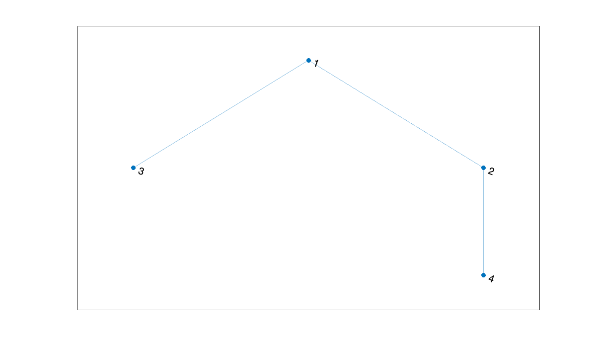
A “buckyball” is an allotrope of carbon atoms with the same connection structure as a soccer ball.
plot(graph(bucky))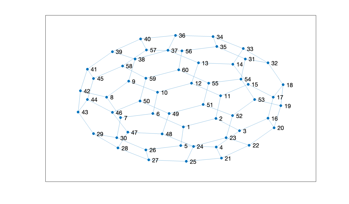
Example 7.1.5
MATLAB ships with a few test images to play with.
A = imread('peppers.png');
color_size = size(A)Use imshow to display the image.
imshow(A)
The image has three layers or channels for red, green, and blue. We can deal with each layer as a matrix, or (as below) convert it to a single matrix indicating shades of gray from black (0) to white (255). Either way, we have to explicitly convert the entries to floating-point values rather than integers.
A = im2gray(A);   % collapse from 3 dimensions to 2
gray_size = size(A)
imshow(A)Before we can do any numerical computation, we need to convert the image to a matrix of floating-point numbers.
A = double(A);7.2 Eigenvalue decomposition
Example 7.2.2
The eig function with one output argument returns a vector of the eigenvalues of a matrix.
A = pi * ones(2, 2);
lambda = eig(A)With two output arguments given, eig returns a matrix eigenvectors and a diagonal matrix with the eigenvalues.
[V, D] = eig(A)We can check the fact that this is an EVD.
norm( A - V*D/V ) % / V is like * inv(V)If the matrix is not diagonalizable, no message is given, but V will be singular. The robust way to detect that circumstance is via .
A = [-1 1; 0 -1];
[V, D] = eig(A)cond(V)Even in the nondiagonalizable case, holds.
norm(A * V - V * D)Example 7.2.3
We first define a hermitian matrix. Note that the ' operation is the adjoint and includes complex conjugation.
n = 7;
A = randn(n, n) + 1i * randn(n, n);
A = (A + A') / 2;
We confirm that the matrix is normal by checking that (to within roundoff).
[V, D] = eig(A);
lambda = diag(D);
cond(V)Now we perturb and measure the effect on the eigenvalues. The Bauer–Fike theorem uses absolute differences, not relative ones. Note: since the ordering of eigenvalues can change, we look at all pairwise differences and take the minima.
E = randn(n, n) + 1i * randn(n, n);
E = 1e-8 * E / norm(E);
dd = eig(A + E);
dist = [];
for j = 1:n
    dist = [dist; min(abs(dd - lambda(j)))];
end
distAs promised, the perturbations in the eigenvalues do not exceed the normwise perturbation to the original matrix.
Now we see what happens for a triangular matrix.
n = 20;
x = (1:n)';
A = triu(x * ones(1, n));
A(1:5, 1:5)This matrix is not at all close to normal.
[V, D] = eig(A);
lambda = diag(D);
cond(V)As a result, the eigenvalues can change by a good deal more.
E = randn(n, n) + 1i * randn(n, n);
E = 1e-8 * E / norm(E);
dd = eig(A + E);
dist = -Inf;
for j = 1:n
    dist = max(dist, min(abs(dd - lambda(j))));
end
fprintf("max change in eigenvalues: %.2e", dist)
fprintf("Bauer-Fike upper bound: %.2e", cond(V) * norm(E))
max change in eigenvalues: 6.84e-01Bauer-Fike upper bound: 6.15e+01If we plot the eigenvalues of many perturbations, we get a cloud of points that roughly represents all the possible eigenvalues when representing this matrix with single-precision accuracy.
clf
plot(lambda, 0*lambda, 'o')
axis equal; hold on
for k = 1:60
    E = randn(n, n) + 1i * randn(n, n);
    E = eps(single(1)) * E / norm(E);
    dd = eig(A + E);
    plot(real(dd), imag(dd), 'k.', markersize=2)
end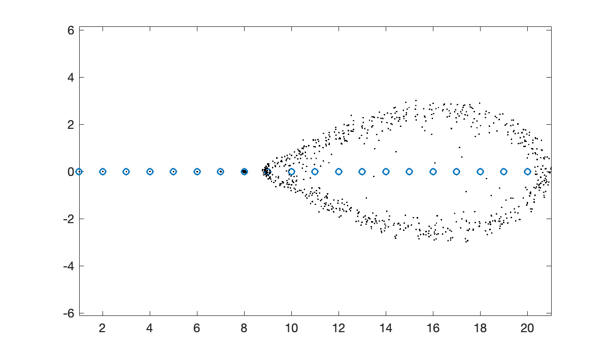
The plot shows that some eigenvalues are much more affected than others. This situation is not unusual, but it is not explained by the Bauer–Fike theorem.
Example 7.2.4
Let’s start with a known set of eigenvalues and an orthogonal eigenvector basis.
D = diag([-6, -1, 2, 4, 5]);
[V, R]= qr(randn(5, 5));    % V is unitary
A = V * D * V';sort(eig(A))Now we will take the QR factorization and just reverse the factors.
[Q, R] = qr(A);
A = R * Q;
It turns out that this is a similarity transformation, so the eigenvalues are unchanged.
sort(eig(A))What’s remarkable, and not elementary, is that if we repeat this transformation many times, the resulting matrix converges to .
for k = 1:40
    [Q, R] = qr(A);
    A = R * Q;
end
format short e
A7.3 Singular value decomposition
Example 7.3.4
We verify some of the fundamental SVD properties using the built-in svd function.
A = vander(1:5);
A = A(:, 1:4)[U, S, V] = svd(A);
disp(sprintf("U is %d by %d. S is %d by %d. V is %d by %d.\n", size(U), size(S), size(V)))U is 5 by 5. S is 5 by 4. V is 4 by 4.
We verify the orthogonality of the singular vectors as follows:
norm(U' * U - eye(5))
norm(V' * V - eye(4))Here is verification of the connections between the singular values, norm, and condition number.
s = diag(S);
norm_A = norm(A)
sigma_max = s(1)cond_A = cond(A)
sigma_ratio = s(1) / s(end)7.4 Symmetry and definiteness
Example 7.4.1
We will use a symmetric matrix with a known EVD and eigenvalues equal to the integers from 1 to 20.
n = 20;
lambda = 1:n;
D = diag(lambda);
[V, ~] = qr(randn(n, n));    % get a random orthogonal V
A = V * D * V';
The Rayleigh quotient is a scalar-valued function of a vector.
R = @(x) (x' * A * x) / (x' * x);The Rayleigh quotient evaluated at an eigenvector gives the corresponding eigenvalue.
format long
R(V(:, 7))If the input to he Rayleigh quotient is within a small δ of an eigenvector, its output is within of the corresponding eigenvalue. In this experiment, we observe that each additional digit of accuracy in an approximate eigenvector gives two more digits to the eigenvalue estimate coming from the Rayleigh quotient.
delta = 1 ./ 10 .^ (1:5)';
dif = zeros(size(delta));
for k = 1:length(delta)
    e = randn(n, 1);
    e = delta(k) * e / norm(e);
    x = V(:, 6) + e;
    dif(k) = R(x) - lambda(6);
end
disp(table(delta, dif, variablenames=["perturbation size", "R(x) - lambda"]))
perturbation size R(x) - lambda
_________________ ____________________
0.1 0.0452326077930536
0.01 0.000323511790824682
0.001 7.21675393666743e-06
0.0001 2.80162018029273e-08
1e-05 4.27677449010844e-10
7.5 Dimension reduction
Example 7.5.1
We make an image from some text, then reload it as a matrix.
clf
tobj = text(0, 0,'Hello world','fontsize',44);
ex = get(tobj, 'extent');
axis([ex(1) ex(1) + ex(3) ex(2) ex(2) + ex(4)]), axis off
exportgraphics(gca, 'hello.png', resolution=300)
A = imread('hello.png');
A = double(im2gray(A));
size_A = size(A)Next we show that the singular values decrease until they reach zero (more precisely, until they are about times the norm of the matrix) at around .
[U, S, V] = svd(A);
sigma = diag(S);
semilogy(sigma, '.')
title('singular values'), axis tight
xlabel('i'), ylabel('\sigma_i')
r = find(sigma / sigma(1) > 10*eps, 1, 'last')The rapid decrease suggests that we can get fairly good low-rank approximations.
for i = 1:4
    subplot(2, 2, i)
    k = 2*i;
    Ak = U(:, 1:k) * S(1:k, 1:k) * V(:, 1:k)';
    imshow(Ak, [0, 255])
    title(sprintf('rank = %d', k))
end
Consider how little data is needed to reconstruct these images. For rank-9, for instance, we have 9 left and right singular vectors plus 9 singular values, for a compression ratio of better than 12:1.
[m, n] = size(A);
full_size = m * n;
compressed_size = 8 * (m + n + 1);
fprintf("compression ratio: %.1f", full_size / compressed_size)
compression ratio: 14.9Example 7.5.2
This matrix describes the votes on bills in the 111th session of the United States Senate. (The data set was obtained from [https://
load votingIf we visualize the votes (yellow is “yea,” blue is “nay”), we can see great similarity between many rows, reflecting party unity.
clf
imagesc(A)
colormap parula
title('Votes in 111th U.S. Senate')
ylabel(('senator'),  xlabel('bill'));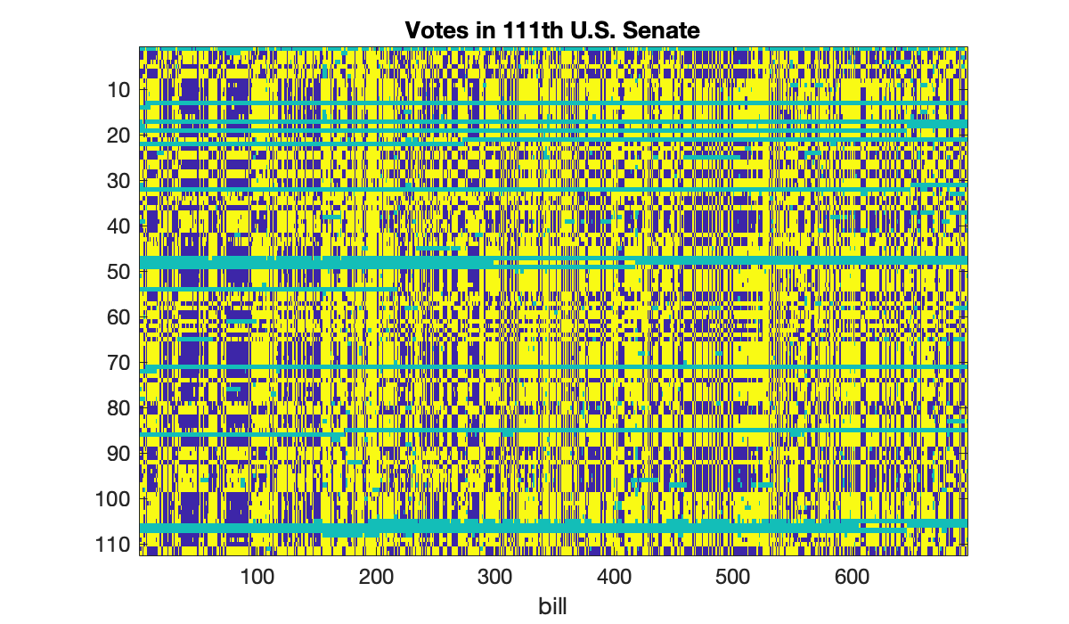
Error using xyzlabel (line 4)
Incorrect number of inputs for property-value pairs.

Error in ylabel (line 7)
    xyzlabel("YLabel", varargin);
We use (7.5.4) to quantify the decay rate of the values.
[U, S, V] = svd(A);
sigma = diag(S);
tau = cumsum(sigma.^2) / sum(sigma.^2);
plot(tau(1:16), 'o')
xlabel('k'),  ylabel('\tau_k')
title(('Fraction of singular value energy'));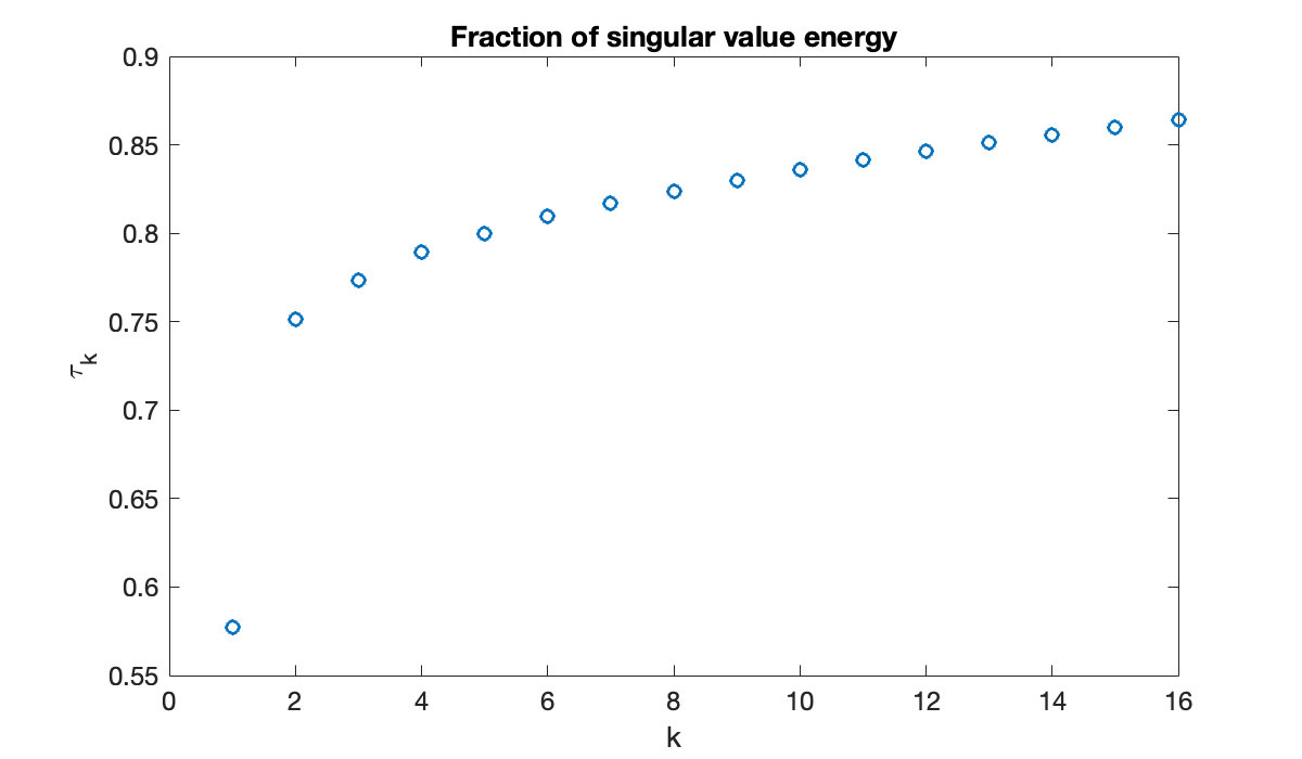
The first and second singular triples contain about 58% and 17%, respectively, of the energy of the matrix. All others have far less effect, suggesting that the information is primarily two-dimensional. The first left and right singular vectors also contain interesting structure.
subplot(211), plot(U(:, 1), '.')
xlabel('senator number'), title('left singular vector')
subplot(212), plot(V(:, 1), '.')
xlabel('bill number'), title(('right singular vector'));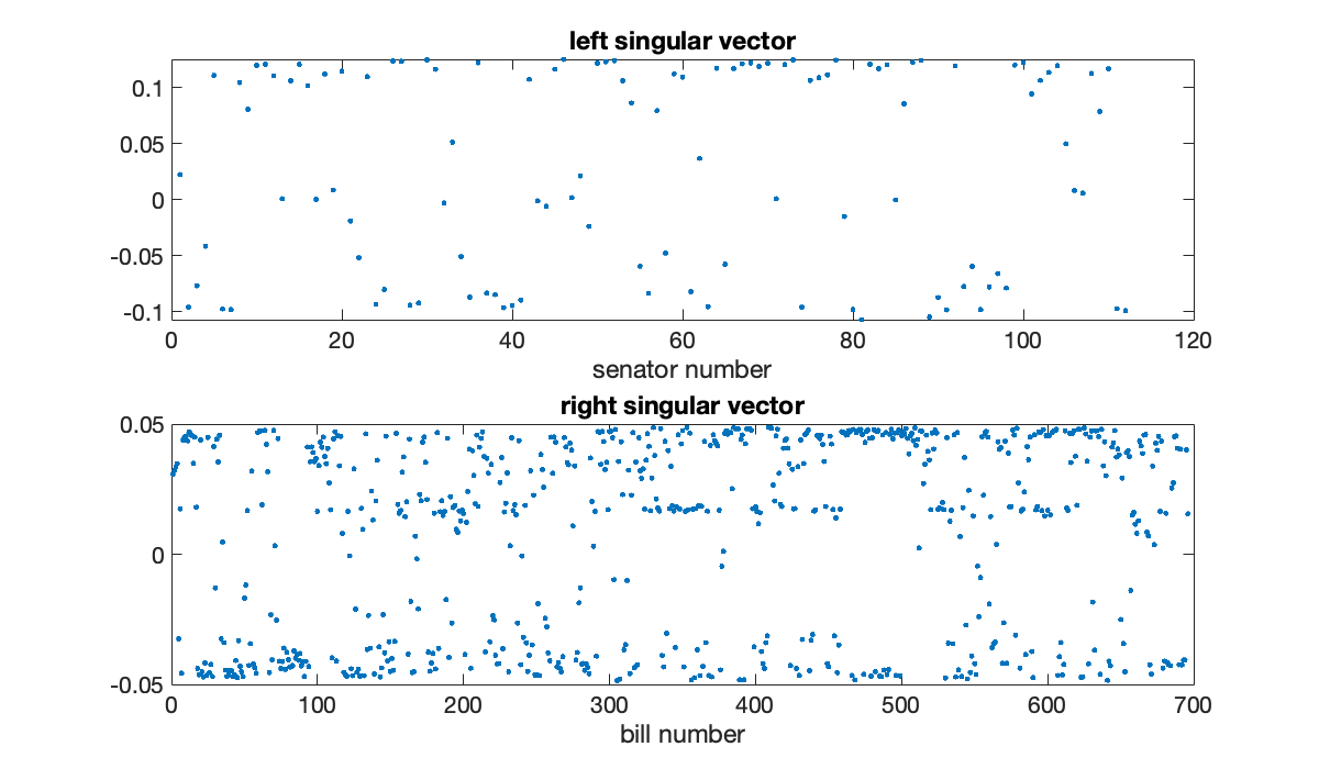
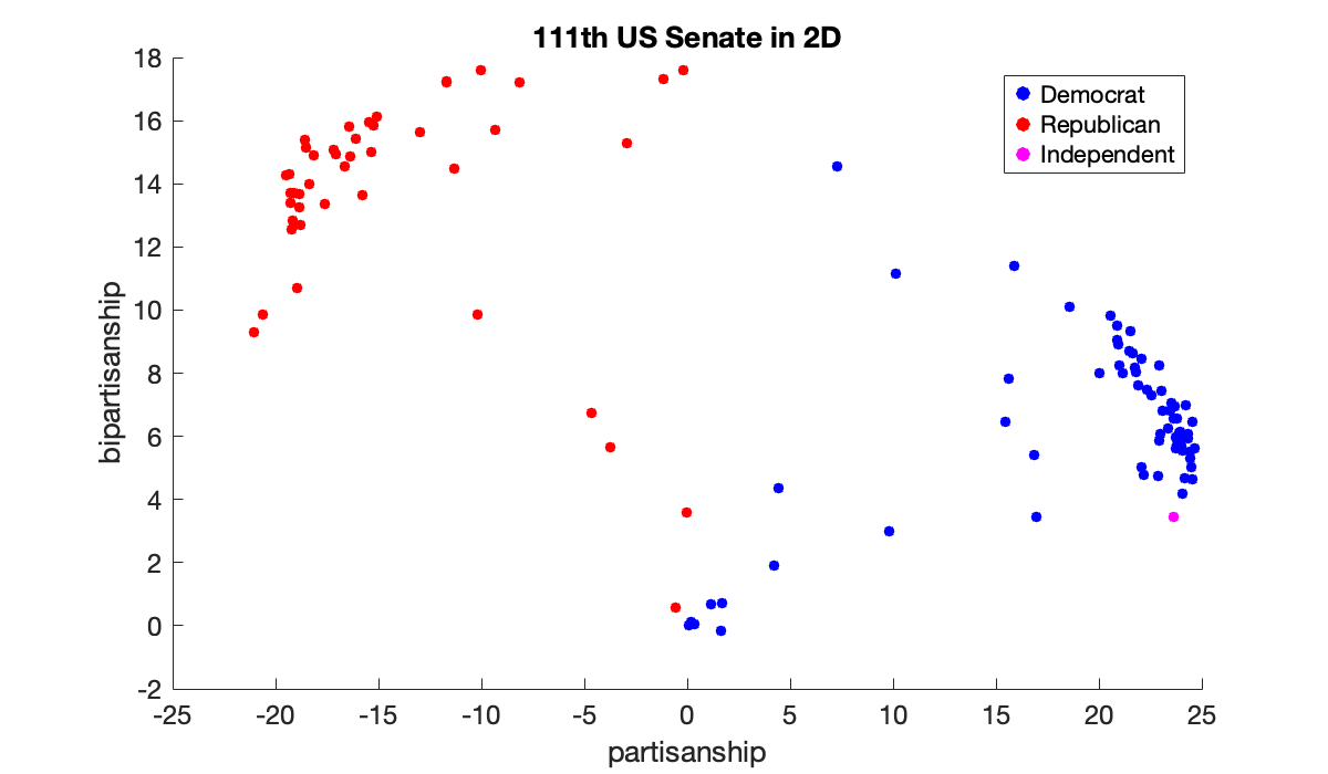
Both vectors have values greatly clustered near for a constant . These can be roughly interpreted as how partisan a particular senator or bill was, and for which political party. Projecting the senators’ vectors into the first two -coordinates gives a particularly nice way to reduce them to two dimensions. Political scientists label these dimensions partisanship and bipartisanship. Here we color them by actual party affiliation (also given in the data file): red for Republican, blue for Democrat, and yellow for independent.
clf
x1 = V(:, 1)'*A';   x2 = V(:, 2)'*A';
scatter(x1(Dem), x2(Dem), 20, 'b'),  hold on
scatter(x1(Rep), x2(Rep), 20, 'r')
scatter(x1(Ind), x2(Ind), 20, 'm')
xlabel('partisanship'),  ylabel('bipartisanship')
legend('Democrat', 'Republican', 'Independent')
title(('111th US Senate in 2D'));