Chapter 11 - Fundamentals of Numerical Computation

Functions¶

Differentiation matrices for periodic end conditions

diffper.m

1
2
3
4
5
6
7
8
9
10
11
12
13
14
15
16
17
18
19
20
21
22
23
24
25
26
27
28
29
function [x,Dx,Dxx] = diffper(n,xspan)
%DIFFPER   Differentiation matrices for periodic end conditions. 
% Input:
%   n      number of subintervals (integer)
%   xspan  endpoints of domain (vector)
% Output:
%   x    equispaced nodes (length n)
%   Dx   matrix for first derivative (n by n)
%   Dxx  matrix for second derivative (n by n)

a = xspan(1);  b = xspan(2);
h = (b-a)/n;
x = a + h*(0:n-1)';   % nodes, omitting the repeated data

% Construct Dx by diagonals, then correct the corners.
dp = 0.5*ones(n-1,1)/h;      % superdiagonal
dm = -0.5*ones(n-1,1)/h;     % subdiagonal
Dx = diag(dm,-1) + diag(dp,1);
Dx(1,n) = -1/(2*h);
Dx(n,1) = 1/(2*h);

% Construct Dxx by diagonals, then correct the corners.
d0 =  -2*ones(n,1)/h^2;      % main diagonal
dp =  ones(n-1,1)/h^2;       % superdiagonal
dm =  dp;                    % subdiagonal
Dxx = diag(dm,-1) + diag(d0) + diag(dp,1);
Dxx(1,n) = 1/(h^2);
Dxx(n,1) = 1/(h^2);

Solution of parabolic PDEs by the method of lines

parabolic.m

1
2
3
4
5
6
7
8
9
10
11
12
13
14
15
16
17
18
19
20
21
22
23
24
25
26
27
28
29
30
31
32
33
34
35
36
37
38
39
40
41
function [x, u] = parabolic(phi, xspan, m, ga, gb, tspan, init)
% PARABOLIC   Solve parabolic PDE by the method of lines.
% Input:
%   phi      defines ∂u/∂t = phi(t, x, u, ∂u/∂x, ∂^2u/∂x^2) 
%   xspan    spatial domain
%   m        number of spatial nodes
%   ga, gb   boundary conditions as functions of u and ∂u/∂x
%   tspan    time interval
%   init     initial condition as a function of x
% Output:       
%   x        spatial nodes (vector)
%   u        function for the solution u(t) at nodes

    [x, Dx, Dxx] = diffcheb(m, xspan);
    int = 2:m;    % indexes of interior nodes

    function u = extend(v)
        function residual = objective(ubc)
            ua = ubc(1);  ub = ubc(2);
            ux = Dx * [ua; v; ub];
            residual = [ga(ua, ux(1)); gb(ub, ux(end))];
        end
        ubc = levenberg(@objective, [0, 0]);
        ubc = ubc(:, end);
        u = [ubc(1); v; ubc(2)];
    end

    function f = mol_ode(t, v, p)
        u = extend(v);
        ux = Dx * u;
        uxx = Dxx * u;
        f = phi(t, x(int), u(int), ux(int), uxx(int));
    end

    ivp = ode(ODEFcn=@mol_ode);
    ivp.InitialTime = tspan(1);
    ivp.InitialValue = init(x(int));
    ivp.Solver = "stiff";
    sol = solutionFcn(ivp, tspan(1), tspan(2));
    u = @(t) extend(sol(t));
end

Examples¶

11.1 Black–Scholes equation¶

Example 11.1.2

We consider the Black–Scholes problem for the following parameter values:

Smax = 8;  T = 6;
K = 3;  sigma = 0.06;  r = 0.08;

We discretize space and time.

m = 200;  h = Smax / m;
x = h * (0:m)';
n = 1000;  tau = T / n;
t = tau * (0:n)';
lambda = tau / h^2;  mu = tau / h;

We set the initial condition and then march forward in time.

V = zeros(m+1, n+1);
V(:, 1) = max(0, x-K);
for j = 1:n
    % Fictitious value from Neumann condition.
    Vfict = 2*h + V(m, j);
    Vj = [ V(:, j); Vfict ];
    % First row is zero by the Dirichlet condition.
    for i = 2:m+1 
        diff1 = (Vj(i+1) - Vj(i-1));
        diff2 = (Vj(i+1) - 2*Vj(i) + Vj(i-1));
        V(i, j+1) = Vj(i) ...
            + (lambda * sigma^2* x(i)^2/2) * diff2  ...
            + (r*mu * x(i))/2 * diff1 - r*tau * Vj(i);
    end 
end

Here is a plot of the solution after every 250 time steps.

index_times = 1:250:n+1;
show_times = t(index_times);
clf
for j = index_times
    str = sprintf("t = %.2f", t(j));
    plot(x, V(:, j), displayname=str) 
    hold on
end
title('Black-Scholes solution')
xlabel('stock price'),  ylabel('option value')
axis tight,  grid on
legend(location="northwest")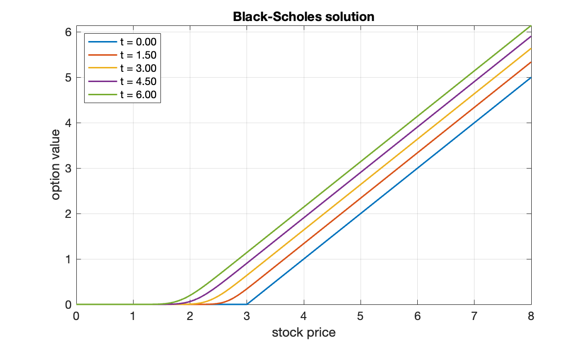

Alternatively, here is an animation of the solution.

clf
plot(x, V(:,1))
hold on,  grid on
axis([0, 8, 0, 6])
title('Black-Scholes solution') 
xlabel('stock price'),  ylabel('option value')
vid = VideoWriter("figures/black-scholes-6.mp4","MPEG-4");
vid.Quality = 85;
open(vid)
for frame = 1:10:n+1
    cla, plot(x, V(:, frame))
    str = sprintf("t = %.2f", t(frame));
    text(0.4, 5.2, str);
    writeVideo(vid, frame2im(getframe(gcf)));
end
close(vid)

The results are easy to interpret, recalling that the time variable really means time until strike. Say you are close to the option’s strike time. If the current stock price is, say, $S=2$ , then it’s not likely that the stock will end up over the strike price $K=3$ , and therefore the option has little value. On the other hand, if presently $S=3$ , then there are good odds that the option will be exercised at the strike time, and you will need to pay a substantial portion of the stock price in order to take advantage. As the time to strike increases, there is an expectation that the stock price is more likely to rise somewhat, making the value of the option larger at each fixed $S$ .

Example 11.1.3

Let’s try to do everything the same as in Demo 11.1.2, but extending the simulation time to $T=8$ .

T = 8;
n = 1000;  tau = T / n;
t = tau*(0:n)';
lambda = tau / h^2;  mu = tau / h;
for j = 1:n
    % Fictitious value from Neumann condition.
    Vfict = 2*h + V(m,j);
    Vj = [ V(:,j); Vfict ];
    % First row is zero by the Dirichlet condition.
    for i = 2:m+1 
        diff1 = (Vj(i+1) - Vj(i-1));
        diff2 = (Vj(i+1) - 2*Vj(i) + Vj(i-1));
        V(i,j+1) = Vj(i) ...
             + (lambda*sigma^2 * x(i)^2/2) * diff2  ...
             + (r*mu * x(i))/2 * diff1 - r*tau * Vj(i);
    end   
end
clf
for j = index_times
    str = sprintf("t = %.2f", t(j));
    plot(x, V(:, j), displayname=str) 
    hold on
end
title('Black-Scholes instability')
xlabel('stock price'),  ylabel('option value')
axis tight,  grid on
legend(location="northwest")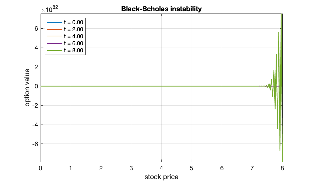

clf
plot(x, V(:,1))
hold on,  grid on
axis([0, 8, 0, 6])
title('Black-Scholes solution...?') 
xlabel('stock price'),  ylabel('option value')
vid = VideoWriter("figures/black-scholes-8.mp4","MPEG-4");
vid.Quality = 85;
open(vid);
for frame = 1:10:n+1
    cla, plot(x, V(:, frame))
    str = sprintf("t = %.2f", t(frame));
    text(0.4, 5.2, str);
    writeVideo(vid, frame2im(getframe(gcf)));
end
close(vid)

This so-called solution is nonsense!

11.2 The method of lines¶

Example 11.2.2

Let’s implement the method of Example 11.2.1 with second-order space semidiscretization.

m = 100;  
[x, Dx, Dxx] = diffper(m, [0, 1]);
Ix = eye(m);

Next we set an initial condition. It isn’t mathematically periodic, but the end values and derivatives are so small that for numerical purposes it may as well be.

tfinal = 0.15;  n = 2400;  
tau = tfinal / n;  t = tau * (0:n)';
U = zeros(m, n+1);
U(:, 1) = exp( -60*(x - 0.5).^2 );

The Euler time stepping simply multiplies the solution vector by the constant matrix in (11.2.6) at each time step. Since that matrix is sparse, we will declare it as such, even though the run-time savings may not be detectable for this small value of $m$ .

A = sparse(Ix + tau * Dxx);
for j = 1:n
    U(:, j+1) = A * U(:,j);
end

index_times = 1:10:31;
show_times = t(index_times);
clf
for j = index_times
    str = sprintf("t = %.2e", t(j));
    plot(x, U(:, j), displayname=str) 
    hold on
end
legend(location="northwest")
xlabel('x'), ylabel('u(x,t)')
title('Heat equation by forward Euler')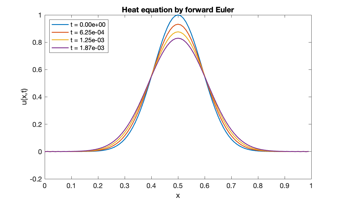

You see above that things seem to start well, with the initial peak widening and shrinking. But then there is a nonphysical growth in the solution.

clf
index_times = 1:101;
plot(x, U(:, 1))
hold on,  grid on
axis([0, 1, -1, 2])
title('Heat equation by forward Euler') 
xlabel('x'),  ylabel('u(x,t)')
vid = VideoWriter("figures/diffusionFE.mp4", "MPEG-4");
vid.Quality = 85;
open(vid);
for frame = index_times
    cla, plot(x, U(:, frame))
    str = sprintf("t = %.3f", t(frame));
    text(0.05, 0.92, str);
    writeVideo(vid, frame2im(getframe(gcf)));
end
close(vid)

The growth in norm is exponential in time.

M = max(abs(U), [], 1);     % max in each column
clf,  semilogy(t, M)
xlabel('t'), ylabel('max_x |u(x,t)|') 
title('Nonphysical growth')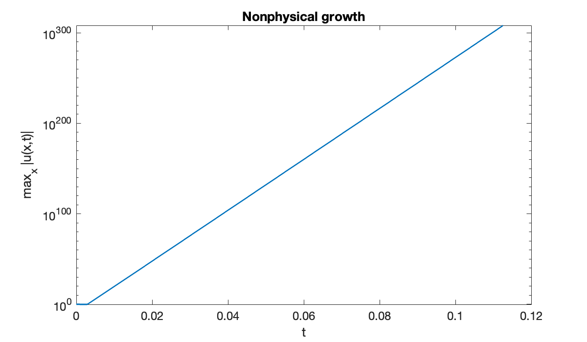

Example 11.2.4

Now we apply backward Euler to the heat equation. Mathematically this means multiplying by the inverse of a matrix, but we interpret that numerically as a linear system solution. We will reuse the setup from Demo 11.2.2.

B = sparse(Ix - tau * Dxx);
[l, u] = lu(B);
for j = 1:n
    U(:, j+1) = u \ (l \ U(:, j));
end

index_times = 1:600:n+1;
show_times = t(index_times);
clf
for j = index_times
    str = sprintf("t = %.2e", t(j));
    plot(x, U(:, j), displayname=str) 
    hold on
end
legend(location="northwest")
xlabel('x'), ylabel('u(x,t)')
title('Heat equation by backward Euler')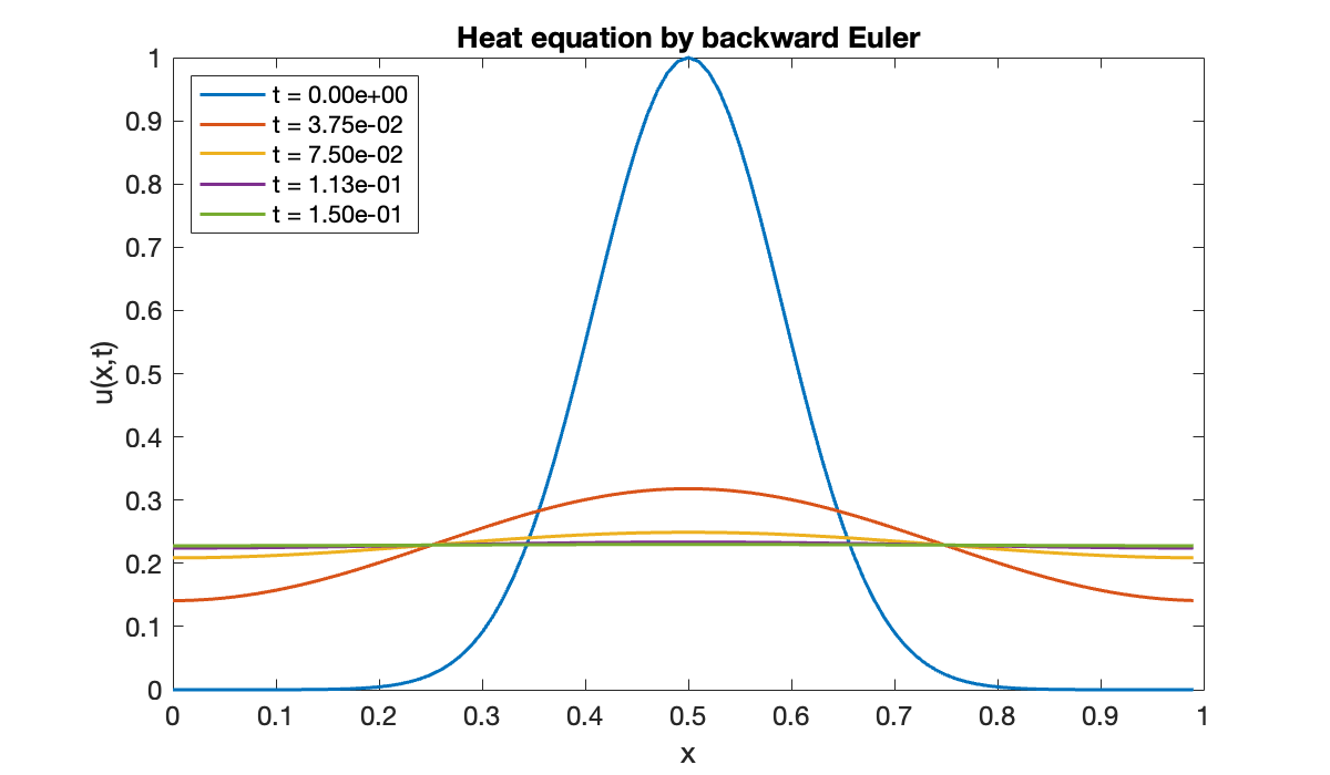

clf
index_times = 1:24:n+1;
plot(x, U(:, 1))
hold on,  grid on
axis([0, 1, -0.25, 1])
title('Heat equation by backward Euler') 
xlabel('x'),  ylabel('u(x,t)')
vid = VideoWriter("figures/diffusionBE.mp4", "MPEG-4");
vid.Quality = 85;
open(vid);
for frame = index_times
    cla, plot(x, U(:, frame))
    str = sprintf("t = %.3f", t(frame));
    text(0.05, 0.92, str);
    writeVideo(vid, frame2im(getframe(gcf)));
end
close(vid)

This solution looks physically plausible, as the large concentration in the center diffuses outward until the solution is essentially constant. Observe that the solution remains periodic in space for all time.

Example 11.2.5

We set up the semidiscretization and initial condition in $x$ just as before.

m = 100;  
[x, Dx, Dxx] = diffper(m, [0, 1]);
Ix = eye(m);
u0 = exp( -60 * (x - 0.5).^2 );

Now, however, we apply a standard solver using solve_ivp to the initial-value problem $\mathbf{u}'=\mathbf{D}_{xx}\mathbf{u}$ .

tfinal = 0.05;
f = @(t, u, p) Dxx * u;
ivp = ode(ODEFcn=f);
ivp.InitialTime = 0;
ivp.InitialValue = u0;
ivp.Solver = 'ode45';
[u, sol] = solutionFcn(ivp, 0, tfinal);

clf
for t = linspace(0, 0.05, 5)
    str = sprintf("t = %.3f", t);
    plot(x, u(t), displayname=str)
    hold on
end
xlabel("x"),  ylabel("u(x,t)")
legend()
title("Heat equation by ode45")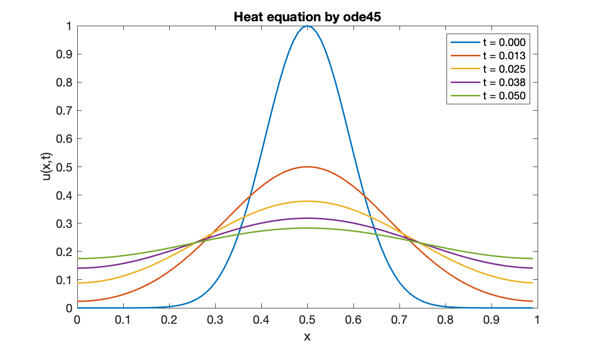

The solution appears to be correct. But the number of time steps that were selected automatically is surprisingly large, considering how smoothly the solution changes.

time_steps_ode45 = length(sol.Time) - 1

Now we apply a different solver called BDF.

ivp.Solver = "ode15s";
[u, sol] = solutionFcn(ivp, 0, tfinal);
time_steps_ode15s = length(sol.Time) - 1

The number of steps selected was reduced by a factor of 20!

11.3 Absolute stability¶

Example 11.3.5

Euler and Backward Euler time-stepping methods were used to solve $\mathbf{u}'=\mathbf{D}_{xx}\mathbf{u}$ .

m = 40;  
[x, Dx, Dxx] = diffper(m, [0, 1]);

The eigenvalues of this matrix are real and negative:

lambda = eig(Dxx);
clf
plot(real(lambda), imag(lambda), 'o')
axis equal, grid on
xlabel('Re \lambda'),  ylabel('Im \lambda')
title('Eigenvalues')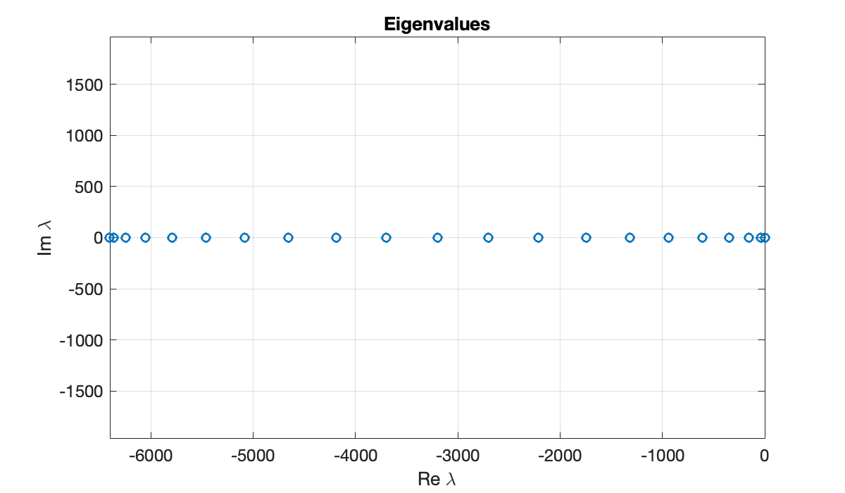

The Euler method is absolutely stable in the region $|\zeta+1| \le 1$ in the complex plane:

phi = linspace(0, 2*pi, 361);
z = exp(1i*phi) - 1;   % unit circle shifted to the left by 1
fill(real(z), imag(z), [.8, .8, 1])
axis equal,  grid on
xlabel('Re \lambda'),  ylabel('Im \lambda')
title('Stability region')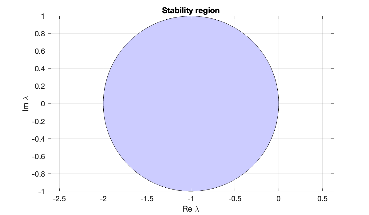

In order to get inside this region, we have to find τ such that $\lambda \tau > -2$ for all eigenvalues λ. This is an upper bound on τ.

lambda_min = min(lambda)
max_tau = -2 / lambda_min

Here we plot the resulting values of $\zeta=\lambda \tau$ .

zeta = lambda * max_tau;
hold on
plot(real(zeta), imag(zeta), 'o')
title('Stability region and \zeta values')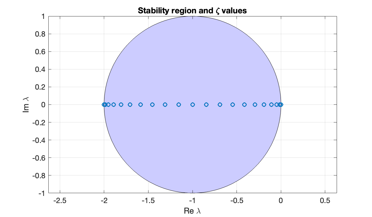

In backward Euler, the region is $|\zeta-1|\ge 1$ . Because they are all on the negative real axis, all of the ζ values will fit no matter what τ is chosen.

clf,  fill([-6, 6, 6, -6],[-6, -6, 6, 6],[.8, .8, 1])
hold on
z = exp(1i*phi) + 1;   % unit circle shifted right by 1
fill(real(z), imag(z), 'w')
plot(real(zeta), imag(zeta), 'o')
axis equal,  axis([-4, 2, -3, 3]), grid on
xlabel('Re \lambda'),  ylabel('Im \lambda')
title('Stability region and \zeta values')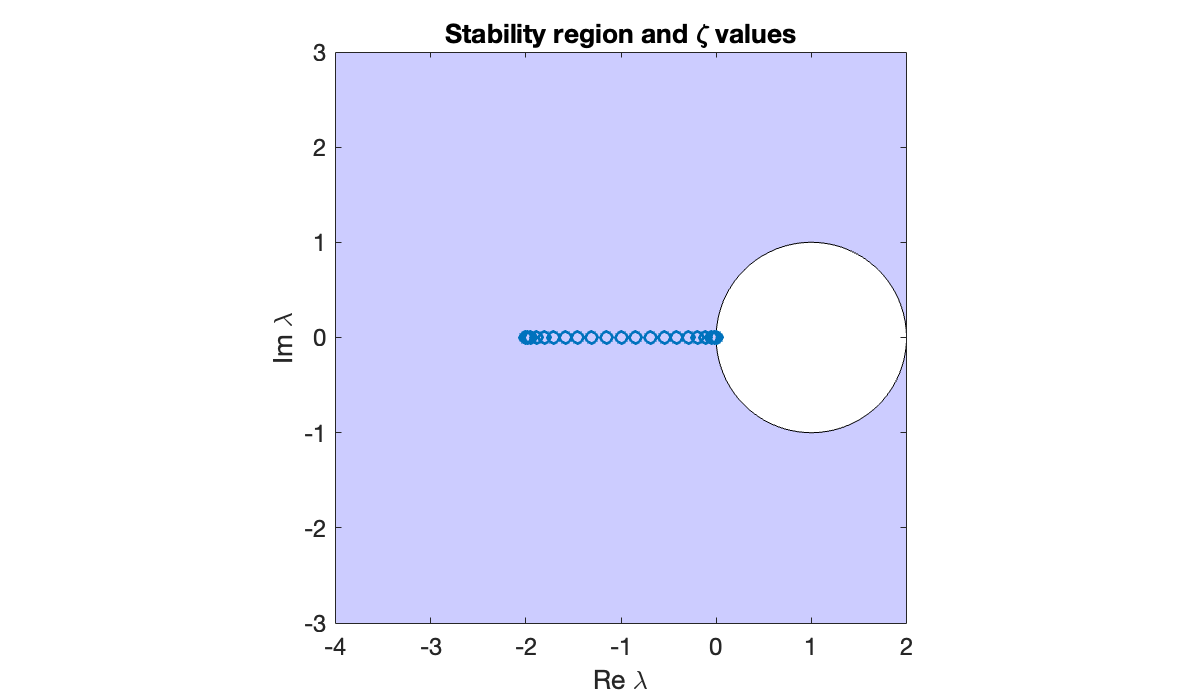

11.4 Stiffness¶

Example 11.4.2

In Example 11.4.1 we derived a Jacobian matrix for the Oregonator model. Here is a numerical solution of the ODE.

q = 8.375e-6;  s = 77.27;  w = 0.161;
f = @(t, u, p) [ s*(u(2)- u(1) * u(2) + u(1) - q * u(1)^2);...
    (-u(2) - u(1) * u(2) + u(3)) / s; ...
    w*(u(1) - u(3)) ];

ivp = ode(ODEFcn=f);
ivp.InitialTime = 0;
ivp.InitialValue = [1; 2; 3];
ivp.Solver = "ode15s";
sol = solve(ivp, 0, 500); 
clf,  semilogy(sol.Time, sol.Solution)
xlabel('t'),  ylabel('u(t)')
title('Oregonator')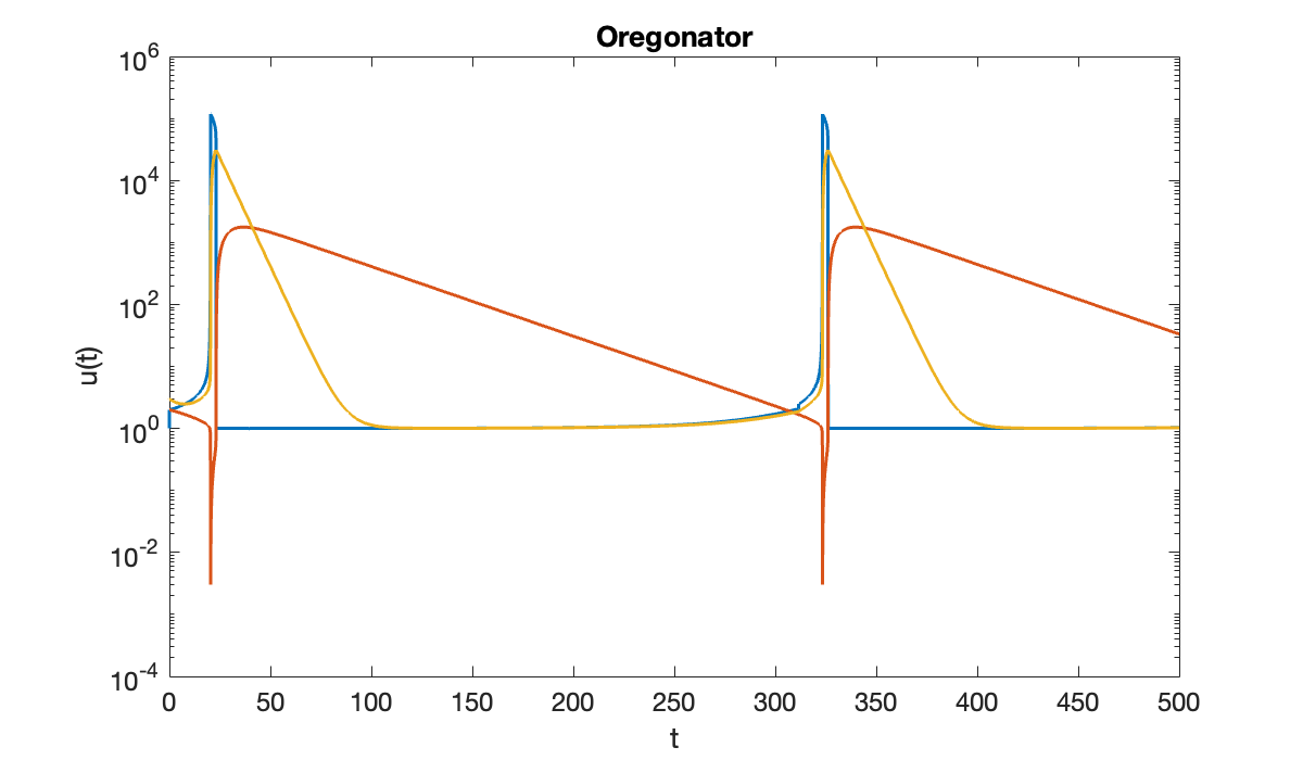

At each value of the numerical solution, we can compute the eigenvalues of the Jacobian. Here we plot all of those eigenvalues in the complex plane.

J = @(u) [ -s*(u(2)+1-2*q*u(1)), s*(1-u(1)), 0; ...
    -u(2)/s, (-1-u(1))/s, 1/s; ...
    w,0,-w];

t = sol.Time;
u = sol.Solution;
lambda = zeros(length(t) - 1, 3);
for j = 1:length(t)-1
    lambda(j, :) = eig(J(u(:, j)));
end
plot3(real(lambda), imag(lambda), t(1:end-1), 'o')
xlabel("Re $\\lambda$"),  ylabel("Im $\\lambda$"),  zlabel("$t$")
title("Oregonator eigenvalues")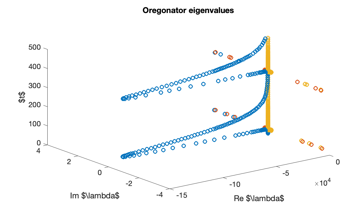

You can see that there is one eigenvalue that ranges over a wide portion of the negative real axis and dominates stability considerations.

Example 11.4.3

The ode15s solver is good for stiff problems and needs few time steps to solve the Oregonator from Demo 11.4.2.

tic,  sol = solve(ivp, 0, 26); 
time_ode15s = toc
num_steps_ode15s = length(sol.Time) - 1

But if we apply Function 6.5.2 to the problem, the step size will be made small enough to cope with the large negative eigenvalue.

tic, [t, u] = rk23(ivp, 0, 26, 1e-5);
time_rk23 = toc
num_steps_rk23 = length(t) - 1

Starting from the eigenvalues of the Jacobian matrix, we can find an effective $\zeta(t)$ by multiplying with the local time step size. The values of $\zeta(t)$ for each time level are plotted below and color coded by component of the diagonalized system.

zeta = zeros(length(t) - 1, 3);
for j = 1:length(t)-1
    lambda = eig(J(u(:, j)));
    zeta(j, :) = (t(j+1) - t(j)) * lambda;
end
plot(zeta, 'o')
axis equal, grid on
xlabel('Re \zeta'),  ylabel('Im \zeta')
title("Oregonator stability")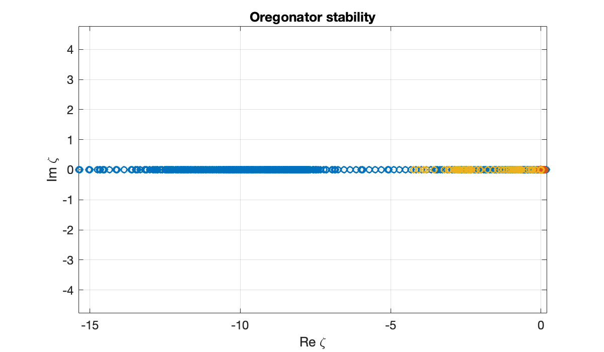

Roughly speaking, the ζ values stay within or close to the RK2 stability region in Figure 11.3.2. Momentary departures from the region are possible, but time stepping repeatedly in that situation would cause instability.

11.5 Boundaries¶

Example 11.5.3

First, we define functions for the PDE and each boundary condition.

phi = @(t, x, u, ux, uxx) uxx;
ga = @(u, ux) u;
gb = @(u, ux) u - 2;

Our next step is to write a function to define the initial condition. This one satisfies the boundary conditions exactly.

init = @(x) 1 + sin(pi * x/2) + 3 * (1 - x.^2) .* exp(-4*x.^2);

Now we can use Function 11.5.2 to solve the problem.

[x, u] = parabolic(phi, [-1, 1], 60, ga, gb, [0, 0.75], init);

clf
for t = 0:0.1:0.5
    str = sprintf("t = %.2f", t);
    plot(x, u(t), displayname=str)
    hold on
end
xlabel("x"),  ylabel("u(x,t)")
legend()
title("Heat equation with Dirichlet boundaries")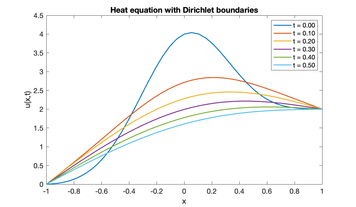

clf
plot(x, u(0))
hold on,  grid on
axis([-1, 1, 0, 4.2])
title('Heat equation with Dirichlet boundaries') 
xlabel('x'),  ylabel('u(x,t)')
vid = VideoWriter("figures/boundaries-heat.mp4", "MPEG-4");
vid.Quality = 85;
open(vid);
for t = linspace(0, 0.75, 201)
    cla, plot(x, u(t))
    str = sprintf("t = %.3f", t);
    text(-0.9, 3.8, str);
    writeVideo(vid, frame2im(getframe(gcf)));
end
close(vid)

Example 11.5.4

phi = @(t, x, u, ux, uxx) u.^2 + uxx;
ga = @(u, ux) u;
gb = @(u, ux) ux;

init = @(x) 400 * x.^4 .* (1 - x).^2;
[x, u] = parabolic(phi, [0, 1], 60, ga, gb, [0, 0.1], init);

clf
plot(x, u(0))
hold on,  grid on
axis([0, 1, 0, 10])
title("Heat equation with source")
xlabel('x'),  ylabel('u(x,t)')
vid = VideoWriter("figures/boundaries-source.mp4", "MPEG-4");
vid.Quality = 85;
open(vid);
for t = linspace(0, 0.1, 101)
    cla, plot(x, u(t))
    str = sprintf("t = %.3f", t);
    text(0.05, 9.2, str);
    writeVideo(vid, frame2im(getframe(gcf)));
end
close(vid)

Example 11.5.5

K = 3;  sigma = 0.06;  r = 0.08;  Smax = 8;
phi = @(t, x, u, ux, uxx) sigma.^2/2 * (x.^2 .* uxx) + r * x.*ux - r*u;
ga = @(u, ux) u;
gb = @(u, ux) ux - 1;

init = @(x) max(0, x - K);
[x, u] = parabolic(phi, [0, Smax], 80, ga, gb, [0, 15], init);

clf
plot(x, u(0))
hold on,  grid on
axis([0, Smax, -0.1, 8])
title("Black–Scholes equation with boundaries")
xlabel('x'),  ylabel('u(x,t)')
vid = VideoWriter("figures/boundaries-bs.mp4", "MPEG-4");
vid.Quality = 85;
open(vid);
for t = linspace(0, 15, 151)
    cla, plot(x, u(t))
    str = sprintf("t = %.1f", t);
    text(0.5, 7.1, str);
    writeVideo(vid, frame2im(getframe(gcf)));
end
close(vid)

Recall that $u$ is the value of the call option, and time runs backward from the strike time. The longer the horizon, the more value the option has due to anticipated growth in the stock price.