Chapter 12 - Fundamentals of Numerical Computation

Examples¶

12.1 Traffic flow¶

In the following definition we allow the velocity $c$ to be specified as a parameter.

[x, Dx, Dxx] = diffper(300, [-4, 4]);
f = @(t, u, c) -c * (Dx*u);
ivp = ode(ODEFcn=f);
ivp.Parameters = 2;
ivp.InitialTime = 0;
ivp.RelativeTolerance = 1e-5;

The following initial condition isn’t mathematically periodic, but the deviation is less than machine precision. We specify RK4 as the solver.

u_init = 1 + exp(-3*x.^2);
ivp.InitialValue = u_init;
t = linspace(0, 3, 201);
sol = solve(ivp, t);
U = sol.Solution;

waterfall(x, t(1:5:end), U(:, 1:5:end)')
view(-13, 65)
xlabel('x'), ylabel('t'), zlabel('u(x,t)')
title('Advection equation')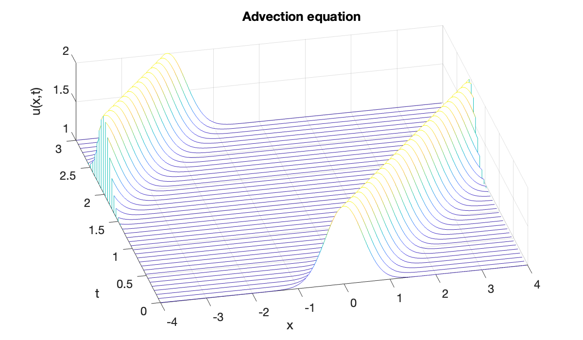

An animation shows the solution nicely. The bump moves with speed 2 to the right, reentering on the left as it exits to the right because of the periodic conditions.

clf
plot(x, U(:, 1))
hold on,  grid on
axis([-4, 4, 0.9, 2.1])
title('Advection equation with periodic boundary') 
xlabel('x'),  ylabel('u(x,t)')
vid = VideoWriter("figures/advection-periodic.mp4","MPEG-4");
vid.Quality = 85;
open(vid);
for frame = 1:length(t)
    cla, plot(x, U(:, frame))
    str = sprintf("t = %.2f", t(frame));
    text(-3.5, 1.9, str);
    writeVideo(vid, frame2im(getframe(gcf)));
end
close(vid)

Example 12.1.2

The following are parameters and a function relevant to defining the problem.

rho_c = 1080;  rho_m = 380;  q_m = 10000;
Q0prime = @(rho) 4*q_m*rho_c^2 * (rho_c - rho_m) * rho_m ...
    *(rho_m - rho) ./ ((rho_c - 2*rho_m) * rho + rho_c * rho_m).^3;
ep = 0.02;

Here we create a discretization on $m=800$ points.

[x, Dx, Dxx] = diffper(800, [0, 4]);

Next we define the ODE resulting from the method of lines.

odefun = @(t, rho) -Q0prime(rho) .* (Dx*rho) + ep * (Dxx*rho);
ivp = ode(ODEFcn=odefun);
ivp.InitialTime = 0;
ivp.RelativeTolerance = 1e-5;

Our first initial condition has moderate density with a small bump. Because of the diffusion present, we use a stiff solver for the IVP.

rho_init = 400 + 10 * exp(-20*(x-3).^2);
ivp.InitialValue = rho_init;

t = linspace(0, 1, 101);
sol = solve(ivp, t);
RHO = sol.Solution;

clf
for plot_idx = 1:20:101
    str = sprintf("t = %.2f", t(plot_idx));
    plot(x, RHO(:, plot_idx), displayname=str)
    hold on
end
xlabel('x'),  ylabel('car density')
title('Traffic flow') 
legend(location="northwest")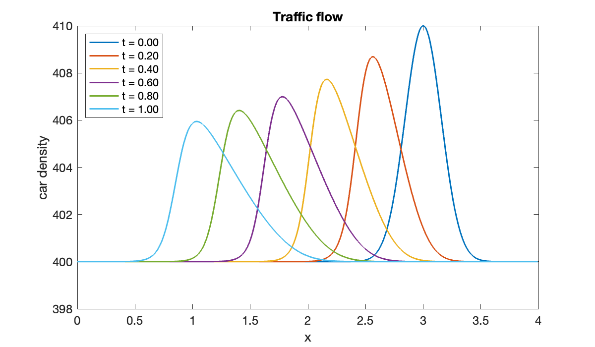

The bump slowly moves backward on the roadway, spreading out and gradually fading away due to the presence of diffusion.

clf
plot(x, RHO(:, 1))
hold on,  grid on
axis([0, 4, 398, 410])
title('Traffic flow') 
xlabel('x'),  ylabel('u(x,t)')
vid = VideoWriter("figures/traffic-small.mp4","MPEG-4");
vid.Quality = 85;
open(vid);
for frame = 1:length(t)
    cla, plot(x, RHO(:, frame))
    str = sprintf("t = %.2f", t(frame));
    text(0.2, 409, str);
    writeVideo(vid, frame2im(getframe(gcf)));
end
close(vid)

Now we use an initial condition with a larger bump. Note that the scale on the $y$ -axis is much different for this solution.

rho_init = 400 + 80 * exp( -16*(x - 3).^2 );
ivp.InitialValue = rho_init;
t = linspace(0, 0.5, 81);
sol = solve(ivp, t);
RHO = sol.Solution;

clf
for plot_idx = 1:16:81
    str = sprintf("t = %.2f", t(plot_idx));
    plot(x, RHO(:, plot_idx), displayname=str)
    hold on
end
xlabel('x'),  ylabel('car density')
title('Traffic jam') 
legend(location="northwest")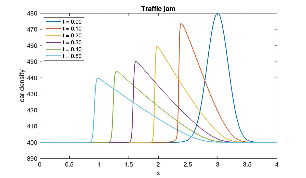

clf
plot(x, RHO(:, 1))
hold on,  grid on
axis([0, 4, 395, 480])
title('Traffic jam') 
xlabel('x'),  ylabel('u(x,t)')
vid = VideoWriter("figures/traffic-jam.mp4", "MPEG-4");
vid.Quality = 85;
open(vid);
for frame = 1:length(t)
    cla, plot(x, RHO(:, frame))
    str = sprintf("t = %.2f", t(frame));
    text(0.2, 470, str);
    writeVideo(vid, frame2im(getframe(gcf)));
end
close(vid)

In this case the density bump travels backward along the road. It also steepens on the side facing the incoming traffic and decreases much more slowly on the other side. A motorist would experience this as an abrupt increase in density, followed by a much more gradual decrease in density and resulting gradual increase in speed. (You also see some transient, high-frequency oscillations. These are caused by instabilities, as we discuss in simpler situations later in this chapter.)

12.2 Upwinding and stability¶

Example 12.2.3

[x, Dx] = diffper(400, [0, 1]);
c = 2;  
ivp = ode(ODEFcn = @(t, u) -c * (Dx*u));
ivp.RelativeTolerance = 1e-5;
ivp.InitialTime = 0;
u_init = exp( -80*(x - 0.5).^2 );
ivp.InitialValue = u_init;

[u, sol] = solutionFcn(ivp, 0, 2);

clf
t = linspace(0, 2, 81);
contour(x, t, u(t)', 12)
xlabel('x'),  ylabel('t')
title('Linear advection')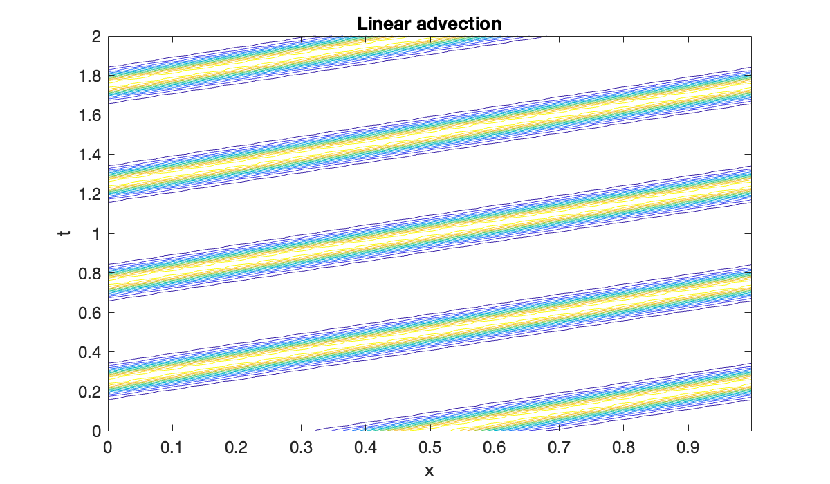

In the space-time plot above, you can see the initial hump traveling rightward at constant speed. It fully traverses the domain once for each integer multiple of $t=1/2$ .

If we cut $h$ by a factor of 2 (i.e., double $m$ ), then the CFL condition suggests that the time step should be cut by a factor of 2 also.

num_steps_400 = length(sol.Time) - 1

[x, Dx] = diffper(800, [0, 1]);
ivp.ODEFcn = @(t, u) -c * (Dx*u);
ivp.InitialValue = exp( -80*(x - 0.5).^2 );
[u, sol] = solutionFcn(ivp, 0, 2);

num_steps_800 = length(sol.Time) - 1
ratio = num_steps_800 / num_steps_400

Example 12.2.6

If we solve advection over $[0,1]$ with velocity $c=-1$ , the right boundary is in the upwind/inflow direction. Thus a well-posed boundary condition is $u(1,t)=0$ .

We’ll pattern a solution after Function 11.5.2. Since $u(x_m,t)=0$ , we define the ODE interior problem (11.5.4) for $\mathbf{v}$ without $u_m$ . For each evaluation of $\mathbf{v}'$ , we must extend the data back to $x_m$ first.

m = 100;  c = -1;
[x, Dx] = diffmat2(m, [0, 1]);
chop = @(u) u(1:m);  
extend = @(v) [v; 0];
odefun = @(t, v) -c * chop( Dx * extend(v) );
ivp = ode(ODEFcn = odefun);
ivp.RelativeTolerance = 1e-5;
ivp.InitialTime = 0;

Now we solve for an initial condition that has a single hump.

u_init = exp( -80*(x - 0.5).^2 );
ivp.InitialValue = chop(u_init);
sol = solutionFcn(ivp, 0, 1);
u = @(t) [sol(t); zeros(1, length(t))];    % extend to zero at right

t = linspace(0, 1, 81);
clf,  contour(x, t, u(t)', 0.15:0.2:1)
xlabel x,  ylabel t
title('Advection with inflow BC')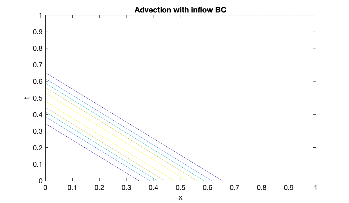

We find that the hump gracefully exits out the downwind end.

clf
plot(x, u(0))
hold on
axis([0, 1, -0.05, 1.05])
title('Advection with inflow BC') 
xlabel('x'),  ylabel('u(x,t)')
vid = VideoWriter("figures/advection-inflow.mp4", "MPEG-4");
vid.Quality = 85;
open(vid);
for frame = 1:length(t)
    cla, plot(x, u(t(frame)))
    str = sprintf("t = %.2f", t(frame));
    text(0.08, 0.85, str);
    writeVideo(vid, frame2im(getframe(gcf)));
end
close(vid)

If instead of $u(1,t)=0$ we were to try to impose the downwind condition $u(0,t)=0$ , we only need to change the index of the interior nodes and where to append the zero value.

chop = @(u) u(2:m+1);  
extend = @(v) [0; v];
ivp.ODEFcn = @(t, v) -c * chop( Dx * extend(v) );
ivp.InitialValue = chop(u_init);
sol = solutionFcn(ivp, 0, 1);
u = @(t) [zeros(1, length(t)); sol(t)];

contour(x, t, u(t)', 0.15:0.2:1)
xlabel x,  ylabel t
title('Advection with outflow BC')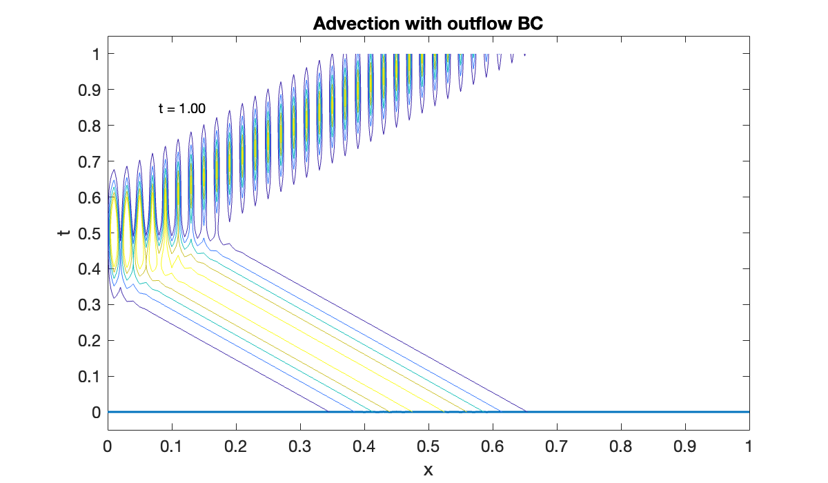

This time, the solution blows up as soon as the hump runs into the boundary because there are conflicting demands there.

clf
plot(x, u(0))
hold on
axis([0, 1, -0.05, 1.05])
title('Advection with outflow BC') 
xlabel('x'),  ylabel('u(x,t)')
vid = VideoWriter("figures/advection-outflow.mp4", "MPEG-4");
vid.Quality = 85;
open(vid);
for frame = 1:45
    cla, plot(x, u(t(frame)))
    str = sprintf("t = %.2f", t(frame));
    text(0.08, 0.85, str);
    writeVideo(vid, frame2im(getframe(gcf)));
end
close(vid)

12.3 Absolute stability¶

Example 12.3.1

For $c=1$ we get purely imaginary eigenvalues.

[x, Dx] = diffper(40, [0, 1]);
lambda = eig(Dx);
clf
scatter(real(lambda), imag(lambda))
axis equal,  grid on
title('Eigenvalues for pure advection')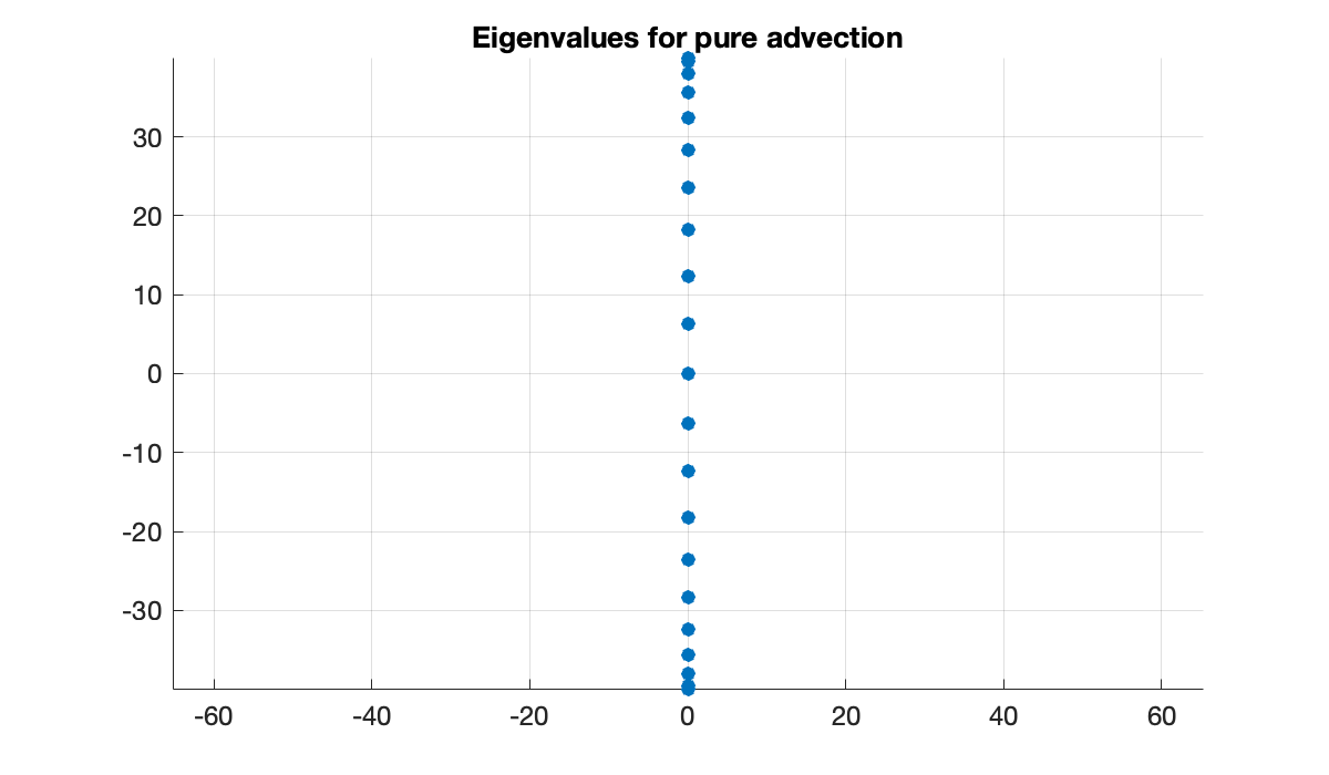

Let’s choose a time step of $\tau=0.1$ and compare to the stability regions of the Euler and backward Euler time steppers (shown as shaded regions):

zc = exp( 1i * linspace(0,2*pi,361)' );    % points on |z|=1
z = zc - 1;    % shift circle left by 1
clf,  fill(real(z), imag(z), [.8, .8, 1])
hold on,  scatter(real(0.1*lambda), imag(0.1*lambda))
axis equal,  axis square
axis([-5, 5, -5, 5]),  grid on
title('Euler')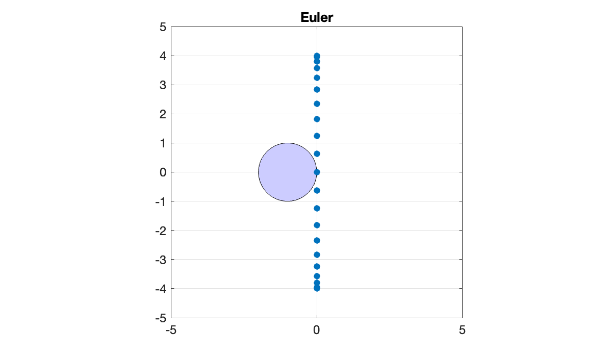

In the Euler case it’s clear that no real value of $\tau>0$ is going to make ζ values fit within the stability region. Any method whose stability region includes none of the imaginary axis is an unsuitable choice for advection.

clf,  fill([-6, 6, 6, -6],[-6, -6, 6, 6], [.8, .8, 1])
z = zc + 1;   % shift circle right by 1
hold on,  scatter(real(0.1*lambda), imag(0.1*lambda))
fill(real(z), imag(z), 'w')
axis equal,  axis square
axis([-5 5 -5 5]),  grid on
title('backward Euler')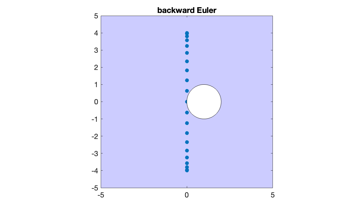

The A-stable backward Euler time stepping tells the exact opposite story: it will be absolutely stable for any choice of the time step τ.

Example 12.3.2

The eigenvalues of advection-diffusion are near-imaginary for $\epsilon\approx 0$ and get closer to the negative real axis as ε increases.

[x, Dx, Dxx] = diffper(40, [0, 1]);
tau = 0.1;
clf
for ep = [0.001 0.01 0.05]
  lambda = eig(-Dx + ep*Dxx);
  str = sprintf("\\epsilon = %.3f", ep);
  scatter(real(tau*lambda), imag(tau*lambda), displayname=str)
  hold on
end
axis equal,  grid on
legend(location='northwest')
title('Eigenvalues for advection-diffusion')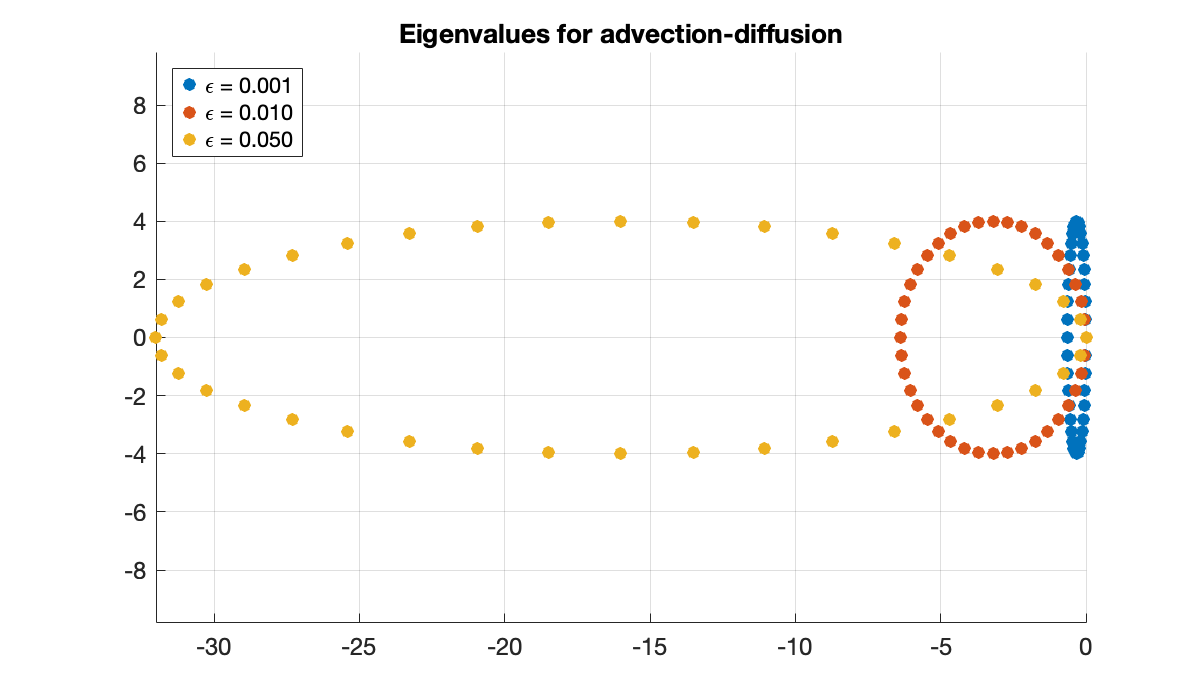

Example 12.3.3

Deleting the last row and column places all the eigenvalues of the discretization into the left half of the complex plane.

[x, Dx, Dxx] = diffcheb(40, [0, 1]);
A = -Dx(2:end, 2:end);    % leave out first row and column
lambda = eig(A);

clf
scatter(real(lambda), imag(lambda))
axis equal,  grid on 
title('Eigenvalues of advection with zero inflow')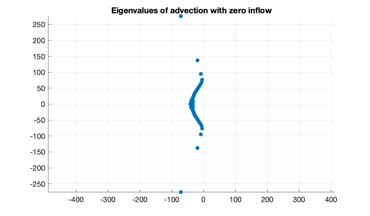

Note that the rightmost eigenvalues have real part at most

max(real(lambda))

Consequently all solutions decay exponentially to zero as $t\to\infty$ . This matches our observation of the solution: eventually, everything flows out of the domain.

12.4 The wave equation¶

Example 12.4.1

c = 2;  m = 200;
[x, Dx] = diffcheb(m, [-1, 1]);

The boundary values of $u$ are given to be zero, so they are not unknowns in the ODEs. Instead they are added or removed as necessary.

chop = @(u) u(2:m);
extend = @(v) [0; v; 0];

The following function computes the time derivative of the system at interior points.

f124wave.m

function dw_dt = wave(t, w, param)
    [c, m, Dx, chop, extend] = param{:};
    u = extend(w(1:m-1));
    z = w(m:2*m);
    du_dt = Dx * z;
    dz_dt = c.^2 .* (Dx * u);
    dw_dt = [ chop(du_dt); dz_dt ];
end

Our initial condition is a single hump for $u$ .

u_init = exp( -100*x.^2 );
z_init = -u_init;
w_init = [ chop(u_init); z_init ];

Because the wave equation is hyperbolic, we can use a nonstiff explicit solver.

ivp = ode(ODEFcn=@f124wave);
ivp.InitialTime = 0;
ivp.InitialValue = w_init;
ivp.RelativeTolerance = 1e-4;
ivp.Parameters = {c, m, Dx, chop, extend};
t = linspace(0, 2, 101);
sol = solve(ivp, t);

We plot the results for the original $u$ variable only. Its interior values are at indices 1:m-1 of the composite $\mathbf{w}$ variable.

W = sol.Solution;
n = length(t)-1;
U = [ zeros(1, n+1); W(1:m-1, :); zeros(1, n+1) ];

cmap = zeros(256, 3);
cmap(129:end, 1) = 2/3;
cmap(1:128, 2) = linspace(1, 0, 128);
cmap(129:256, 2) = linspace(0, 1, 128);
cmap(1:128, 3) = linspace(1, 0.5, 128);
cmap(129:256, 3) = linspace(0.5, 1, 128);
cmap = hsv2rgb(cmap);

clf,  contour(x, t, U', 24, linewidth=2)
colormap(cmap),  clim([-1, 1])
xlabel x,  ylabel t
title("Wave equation with boundaries")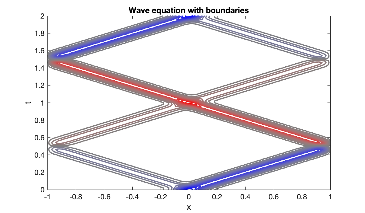

clf
plot(x, U(:, 1))
hold on
axis([-1, 1, -1.05, 1.05])
title("Wave equation with boundaries") 
xlabel('x'),  ylabel('u(x,t)')
vid = VideoWriter("figures/wave-boundaries.mp4", "MPEG-4");
vid.Quality = 85;
open(vid);
for frame = 1:length(t)
    cla, plot(x, U(:, frame))
    str = sprintf("t = %.2f", t(frame));
    text(-0.92, 0.85, str, fontsize=16);
    writeVideo(vid, frame2im(getframe(gcf)));
end
close(vid)

The original hump breaks into two pieces of different amplitudes, each traveling with speed $c=2$ . They pass through one another without interference. When a hump encounters a boundary, it is perfectly reflected, but with inverted shape. At time $t=2$ , the solution looks just like the initial condition.

Example 12.4.2

We now use a wave speed that is discontinuous at $x=0$ .

m = 120;
[x, Dx] = diffcheb(m, [-1, 1]);
c = 1 + (sign(x) + 1) / 2;
chop = @(u) u(2:m);
extend = @(v) [0; v; 0];

u_init = exp( -100*(x + 0.5).^2 );
z_init = -u_init;
ivp.InitialValue = [ chop(u_init); z_init ]; 
ivp.Parameters = {c, m, Dx, chop, extend};
sol = solve(ivp, t);
W = sol.Solution;
U = [ zeros(1, n+1); W(1:m-1, :); zeros(1, n+1) ];

clf,  contour(x, t, U', 24, linewidth=2)
colormap(cmap),  clim([-1, 1])
xlabel x,  ylabel t
title("Wave equation with variable speed")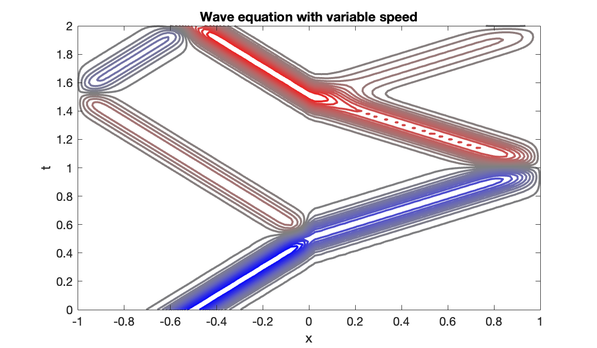

clf
plot(x, U(:, 1))
hold on
axis([-1, 1, -1.05, 1.05])
title("Wave equation with variable speed") 
xlabel('x'),  ylabel('u(x,t)')
vid = VideoWriter("figures/wave-speed.mp4", "MPEG-4");
vid.Quality = 85;
open(vid);
for frame = 1:length(t)
    cla, plot(x, U(:, frame))
    str = sprintf("t = %.2f", t(frame));
    text(-0.92, 0.85, str, fontsize=16);
    writeVideo(vid, frame2im(getframe(gcf)));
end
close(vid)

Each pass through the interface at $x=0$ generates a reflected and transmitted wave. By conservation of energy, these are both smaller in amplitude than the incoming bump.