Functions
Shooting method for a two-point boundary-value problem
1 2 3 4 5 6 7 8 9 10 11 12 13 14 15 16 17 18 19 20 21 22 23 24 25 26 27 28 29 30 31 32 33 34 35 36 37 38 39def shoot(phi, a, b, ga, gb, init): """ shoot(phi, a, b, ga, gb, init) Use the shooting method to solve a two-point boundary value problem. The ODE is u'' = phi(x, u, u') for x in (a,b). The functions ga(u(a), u'(a)) and gb(u(b), u'(b)) specify the boundary conditions. The value init is an initial guess for [u(a), u'(a)]. Return vectors for the nodes, the values of u, and the values of u'. """ # Tolerances for IVP solver and rootfinder. tol = 1e-5 # To be solved by the IVP solver def shootivp(x, y): return np.array([y[1], phi(x, y[0], y[1])]) # Evaluate the difference between computed and target values at x=b. def objective(s): nonlocal x, y # change these values in outer scope x = np.linspace(a, b, 400) # make decent plots on return sol = solve_ivp(shootivp, [a, b], s, atol=tol/10, rtol=tol/10, t_eval=x) x = sol.t y = sol.y residual = np.array([ga(y[0, 0], y[1, 0]), gb(y[0, -1], y[0, -1])]) return residual # Find the unknown quantity at x=a by rootfinding. x, y = [], [] # the values will be overwritten s = levenberg(objective, init, tol) # Don't need to solve the IVP again. It was done within the # objective function already. u = y[0] # solution du_dx = y[1] # derivative return x, u, du_dx
Second-order differentiation matrices
1 2 3 4 5 6 7 8 9 10 11 12 13 14 15 16 17 18 19 20 21 22 23 24 25 26 27 28 29 30 31def diffmat2(n, xspan): """ diffmat2(n, xspan) Compute 2nd-order-accurate differentiation matrices on n+1 points in the interval xspan. Return a vector of nodes, and the matrices for the first and second derivatives. """ a, b = xspan h = (b - a) / n x = np.linspace(a, b, n + 1) # nodes # Define most of Dx by its diagonals. dp = 0.5 / h * np.ones(n) # superdiagonal dm = -0.5 / h * np.ones(n) # subdiagonal Dx = np.diag(dm, -1) + np.diag(dp, 1) # Fix first and last rows. Dx[0, :3] = np.array([-1.5, 2, -0.5]) / h Dx[-1, -3:] = np.array([0.5, -2, 1.5]) / h # Define most of Dxx by its diagonals. d0 = -2 / h**2 * np.ones(n + 1) # main diagonal dp = np.ones(n) / h**2 # superdiagonal and subdiagonal Dxx = np.diag(d0, 0) + np.diag(dp, -1) + np.diag(dp, 1) # Fix first and last rows. Dxx[0, :4] = np.array([2, -5, 4, -1]) / h**2 Dxx[-1, -4:] = np.array([-1, 4, -5, 2]) / h**2 return x, Dx, Dxx
Chebyshev differentiation matrices
1 2 3 4 5 6 7 8 9 10 11 12 13 14 15 16 17 18 19 20 21 22 23 24 25 26 27 28 29 30 31 32def diffcheb(n, xspan): """ diffcheb(n, xspan) Compute Chebyshev differentiation matrices on n+1 points in the interval xspan. Return a vector of nodes, and the matrices for the first and second derivatives. """ x = -np.cos(np.arange(n + 1) * np.pi / n) # nodes in [-1,1] Dx = np.zeros([n + 1, n + 1]) c = np.hstack([2.0, np.ones(n - 1), 2.0]) # endpoint factors # Off-diagonal entries Dx = np.zeros([n + 1, n + 1]) for i in range(n + 1): for j in range(n + 1): if i != j: Dx[i, j] = (-1) ** (i + j) * c[i] / (c[j] * (x[i] - x[j])) # Diagonal entries by the "negative sum trick" for i in range(n + 1): Dx[i, i] = -np.sum([Dx[i, j] for j in range(n + 1) if j != i]) # Transplant to [a,b] a, b = xspan x = a + (b - a) * (x + 1) / 2 Dx = 2 * Dx / (b - a) # Second derivative Dxx = Dx @ Dx return x, Dx, Dxx
Solution of a linear boundary-value problem
1 2 3 4 5 6 7 8 9 10 11 12 13 14 15 16 17 18 19 20 21 22 23 24 25 26def bvplin(p, q, r, xspan, lval, rval, n): """ bvplin(p, q, r, xspan, lval, rval, n) Use finite differences to solve a linear bopundary value problem. The ODE is u''+p(x)u'+q(x)u = r(x) on the interval xspan, with endpoint function values given as lval and rval. There will be n+1 equally spaced nodes, including the endpoints. Return vectors of the nodes and the solution values. """ x, Dx, Dxx = diffmat2(n, xspan) P = np.diag(p(x)) Q = np.diag(q(x)) L = Dxx + P @ Dx + Q # ODE expressed at the nodes # Replace first and last rows using boundary conditions. I = np.eye(n + 1) A = np.vstack([I[0], L[1:-1], I[-1]]) b = np.hstack([lval, r(x[1:-1]), rval]) # Solve the system. u = np.linalg.solve(A, b) return x, u
About the code
Note that there is no need to explicitly form the row-deletion matrix from (10.4.8). Since it only appears as left-multiplying or , we simply perform the row deletions as needed using indexing.
Solution of a nonlinear boundary-value problem
1 2 3 4 5 6 7 8 9 10 11 12 13 14 15 16 17 18 19 20 21 22 23 24 25 26 27 28def bvp(phi, xspan, ga, gb, init): """ bvp(phi, xspan, ga, gb, init) Use finite differences to solve a two-point boundary value problem. The ODE is u'' = phi(x, u, u') for x in (a,b). The functions ga(u(a), u'(a)) and gb(u(b), u'(b)) specify the boundary conditions. The value init is an initial guess for [u(a), u'(a)]. Return vectors for the nodes and the values of u. """ n = len(init) - 1 x, Dx, Dxx = diffmat2(n, xspan) h = x[1] - x[0] def residual(u): # Compute the difference between u'' and phi(x,u,u') at the # interior nodes and appends the error at the boundaries. du_dx = Dx @ u # discrete u' d2u_dx2 = Dxx @ u # discrete u'' f = d2u_dx2 - phi(x, u, du_dx) # Replace first and last values by boundary conditions. f[0] = ga(u[0], du_dx[0]) / h f[n] = gb(u[n], du_dx[n]) / h return f u = levenberg(residual, init.copy()) return x, u[-1]
About the code
The nested function residual uses differentiation matrices computed externally to it, rather than computing them anew on each invocation. As in Function 10.4.1, there is no need to form the row-deletion matrix explicitly. In lines 23--24, we divide the values of and by a factor of . This helps scale the residual components more uniformly and improves the robustness of convergence a bit.
Piecewise linear finite elements for a linear BVP
1 2 3 4 5 6 7 8 9 10 11 12 13 14 15 16 17 18 19 20 21 22 23 24 25 26 27 28 29 30 31 32 33 34 35 36 37 38 39 40 41 42 43 44 45 46 47 48def fem(c, s, f, a, b, n): """ fem(c, s, f, a, b, n) Use a piecewise linear finite element method to solve a two-point boundary value problem. The ODE is (c(x)u')' + s(x)u = f(x) on the interval [a,b], and the boundary values are zero. The discretization uses n equal subintervals. Return vectors for the nodes and the values of u. """ # Define the grid. h = (b - a) / n x = np.linspace(a, b, n + 1) # Templates for the subinterval matrix and vector contributions. Ke = np.array([[1, -1], [-1, 1]]) Me = (1 / 6) * np.array([[2, 1], [1, 2]]) fe = (1 / 2) * np.array([1, 1]) # Evaluate coefficent functions and find average values. cval = c(x) cbar = (cval[:-1] + cval[1:]) / 2 sval = s(x) sbar = (sval[:-1] + sval[1:]) / 2 fval = f(x) fbar = (fval[:-1] + fval[1:]) / 2 # Assemble global system, one interval at a time. K = np.zeros([n - 1, n - 1]) M = np.zeros([n - 1, n - 1]) f = np.zeros(n - 1) K[0, 0] = cbar[0] / h M[0, 0] = sbar[0] * h / 3 f[0] = fbar[0] * h / 2 K[-1, -1] = cbar[-1] / h M[-1, -1] = sbar[-1] * h / 3 f[-1] = fbar[-1] * h / 2 for k in range(1, n - 1): K[k - 1 : k + 1, k - 1 : k + 1] += (cbar[k] / h) * Ke M[k - 1 : k + 1, k - 1 : k + 1] += (sbar[k] * h) * Me f[k - 1 : k + 1] += (fbar[k] * h) * fe # Solve system for the interior values. u = np.linalg.solve(K + M, f) u = np.hstack([0, u, 0]) # put the boundary values into the result return x, u
Examples
10.1 Two-point BVP
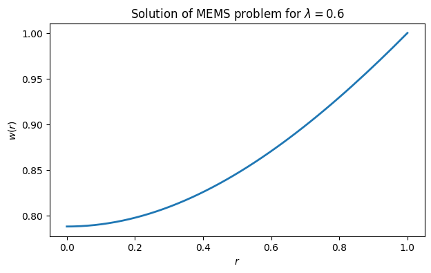
Example 10.1.3
To solve this problem, we have to define functions for the ODE and boundary conditions. The first returns the computed values of and .
lamb = 0.6
def ode(r, y):
    return array([
        y[1],
        lamb / y[0]**2 - y[1] / r
    ])
To encode the boundary conditions , , we define a function for their residual values.
def bc(ya, yb):    # given y(a), y(b)
    return array([
        ya[1],
        yb[0] - 1
    ])
The domain of the mathematical problem is . However, there is a division by in the ODE, so we want to avoid by truncating the domain a bit.
a, b = finfo(float).eps, 1We need one last ingredient that is not part of the mathematical setup: an initial estimate for the solution. As we will see, this plays the same role as initialization in Newton’s method for rootfinding. Here, we try a constant value for each component.
r = linspace(a, b, 50)
y_init = vstack([ones(r.size), zeros(r.size)])
Now we can solve the problem using solve_bvp from scipy.integrate.
from scipy.integrate import solve_bvp
sol = solve_bvp(ode, bc, r, y_init)
print(f"Solved at {sol.x.size} nodes.")
plot(sol.x, sol.y[0])
xlabel("$r$"),  ylabel("$w(r)$")
title("Solution of MEMS problem for $\\lambda=0.6$");
Solved at 998 nodes.
10.2 Shooting
Example 10.2.1
Let’s first examine the shooting approach for the TPBVP from Example 10.1.2 with .
lamb = 0.6
phi = lambda r, w, dw_dr: lamb / w**2 - dw_dr / r
We convert the ODE to a first-order system in order to apply a numerical method. We also have to truncate the domain to avoid division by zero.
f = lambda r, y: hstack([y[1], phi(r, y[0], y[1])])
a, b = finfo(float).eps, 1
The BVP specifies . We can try multiple values for the unknown and plot the solutions.
from scipy.integrate import solve_ivp
t = linspace(a, b, 400)
for w0 in arange(0.4, 1.0, 0.1):
    sol = solve_ivp(f, [a, b], [w0, 0], t_eval=t)
    plot(t, sol.y[0], label=f"$w_0$ = {w0:.1f}")

xlabel("$r$"),  ylabel("$w(r)$")
legend(),  grid(True)
title("Solutions for choices of w(0)");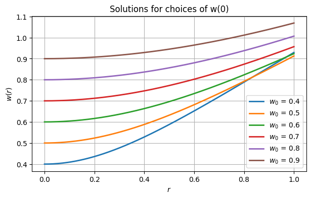
On the graph, it’s the curve starting at that comes closest to the required condition , but it’s a bit too large.
Example 10.2.2
We revisit Demo 10.2.1 but let Function 10.2.1 do the heavy lifting.
lamb = 0.6
phi = lambda r, w, dwdr: lamb / w**2 - dwdr / r
a, b = finfo(float).eps, 1
We specify the given and unknown endpoint values.
ga = lambda w, dw : dw       # w'=0 at left
gb = lambda w, dw : w - 1    # w=1 at right
In this setting, we need to provide initial guesses for and .
init = array([0.8, 0])
r, w, dw_dx = FNC.shoot(phi, a, b, ga, gb, init)
plot(r, w)
title("Shooting solution")
xlabel("$r$"),  ylabel("$w(r)$");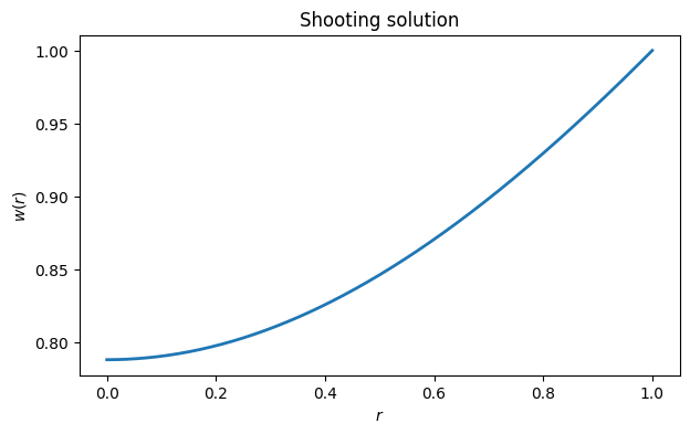
The value of at , meant to be exactly one, was computed to be
print(f"w at right end is {w[-1]}")w at right end is 1.0000010017900354
The accuracy is consistent with the error tolerance used for the IVP solution by shoot. The initial value that gave this solution is
print(f"w at left end is {w[0]}")w at left end is 0.7877599056161069
Example 10.2.3
ga = lambda u, du : u + 1    # u=-1 at left
gb = lambda u, du : u        # u= 0 at right
init = array([-1, 0])
for lamb in range(6, 22, 4):
    phi = lambda x, u, du_dx: lamb**2 * u + lamb**2
    x, u, du_dx = FNC.shoot(phi, 0.0, 1.0, ga, gb, init)
    plot(x, u, label=f"$\\lambda$ = {lamb:.1f}")

xlabel("$x$"),  ylabel("$u(x)$"),  ylim(-1.0, 0.25)
grid(True),  legend(loc="upper left")
title("Shooting instability");
/Users/driscoll/Dropbox/Mac/Documents/GitHub/fnc/python/fncbook/fncbook/chapter04.py:167: UserWarning: Iteration did not find a root.
warnings.warn("Iteration did not find a root.")
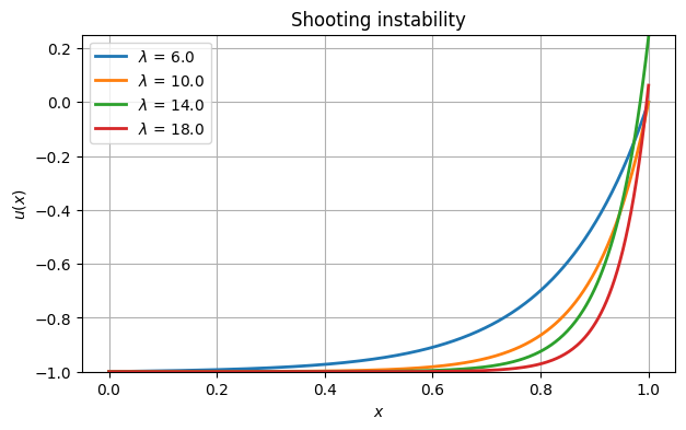
The numerical solutions evidently don’t satisfy the right boundary condition as λ increases, which makes them invalid.
10.3 Differentiation matrices
Example 10.3.1
We test first-order and second-order differentiation matrices for the function over .
f = lambda x: x + exp( sin(4 * x) )For reference, here are the exact first and second derivatives.
df_dx = lambda x: 1 + 4 * exp(sin(4 * x)) * cos(4 * x)
d2f_dx2 = lambda x: 4 * exp(sin(4 * x)) * (4 * cos(4 * x)**2 - 4 * sin(4 * x))
We discretize on equally spaced nodes and evaluate at the nodes.
t, Dx, Dxx = FNC.diffmat2(12, [-1, 1])
y = f(t)
Then the first two derivatives of each require one matrix-vector multiplication.
yx = Dx @ y
yxx = Dxx @ y
The results show poor accuracy for this small value of .
x = linspace(-1, 1, 500)
subplot(2, 1, 1)
plot(x, df_dx(x))
plot(t, yx, "ko")
xlabel("$x$"),  ylabel("$f'(x)$")

subplot(2, 1, 2)
plot(x, d2f_dx2(x))
plot(t, yxx, "ko")
xlabel("$x$"),  ylabel("$f''(x)$");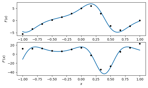
A convergence experiment confirms the order of accuracy. Because we expect an algebraic convergence rate, we use a log-log plot of the errors.
N = array([int(2**k) for k in arange(4, 11.5, 0.5)])
err1 = zeros(len(N))
err2 = zeros(len(N))
for k, n in enumerate(N):
    t, Dx, Dxx = FNC.diffmat2(n, [-1, 1])
    y = f(t)
    err1[k] = norm(df_dx(t) - Dx @ y, inf)
    err2[k] = norm(d2f_dx2(t) - Dxx @ y, inf)

loglog(N, err1, "-o", label="$f'$")
loglog(N, err2, "-o", label="$f''$")
plot(N, 10 * 10 / N**2, "k--", label="2nd order")
xlabel("$n$"),  ylabel("max error")
legend(loc="lower left")
title("Convergence of finite differences");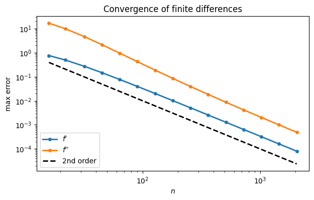
Example 10.3.2
Here is a Chebyshev differentiation matrix.
t, Dx, Dxx = FNC.diffcheb(3, [-1, 1])
print(Dx)
[[-3.16666667 4. -1.33333333 0.5 ]
[-1. 0.33333333 1. -0.33333333]
[ 0.33333333 -1. -0.33333333 1. ]
[-0.5 1.33333333 -4. 3.16666667]]
We again test the convergence rate.
f = lambda x: x + exp(sin(4 * x))
df_dx = lambda x: 1 + 4 * exp(sin(4 * x)) * cos(4 * x)
d2f_dx2 = lambda x: 4 * exp(sin(4 * x)) * (4 * cos(4 * x) ** 2 - 4 * sin(4 * x))

N = range(5, 75, 5)
err1 = zeros(len(N))
err2 = zeros(len(N))
err = zeros((len(N), 2))
for k, n in enumerate(N):
    t, Dx, Dxx = FNC.diffcheb(n, [-1, 1])
    y = f(t)
    err[k, 0] = norm(df_dx(t) - Dx @ y, inf)
    err[k, 1] = norm(d2f_dx2(t) - Dxx @ y, inf)
Since we expect a spectral convergence rate, we use a semi-log plot for the error.
semilogy(N, err, "-o")
xlabel("$n$"), ylabel("max error")
legend(["$f'$", "$f''$"], loc="lower left")
title("Convergence of Chebyshev derivatives");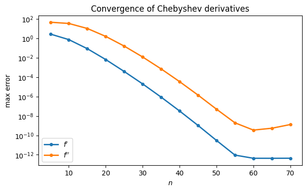
10.4 Collocation for linear problems
Example 10.4.1
exact = lambda x: exp( sin(x) )The problem is presented above in our standard form, so we can identify the coefficient functions in the ODE. Each should be coded as a function.
p = lambda x: -cos(x)
q = sin
r = lambda x: 0 * x    # must be a function
We solve the BVP and compare the result to the exact solution.
x, u = FNC.bvplin(p, q, r, [0, pi/2], 1, exp(1), 25)subplot(2, 1, 1)
plot(x, u)
ylabel("solution"), title("Solution of the BVP")
subplot(2, 1, 2)
plot(x, exact(x) - u, "-o")
ylabel("error");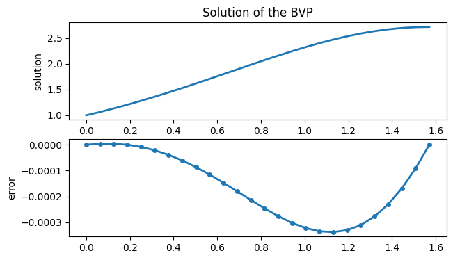
Example 10.4.2
lamb = 10
exact = lambda x: sinh(lamb * x) / sinh(lamb) - 1
The following functions define the ODE.
p = lambda x: zeros(size(x))
q = lambda x: -(lamb**2) * ones(len(x))
r = lambda x: lamb**2 * ones(len(x))
We compare the computed solution to the exact one for increasing .
N = array([int(2 * 10**d) for d in arange(1, 3.1, 0.25)])
err = zeros(len(N))
results = PrettyTable(["n", "error"])
for k, n in enumerate(N):
    x, u = FNC.bvplin(p, q, r, [0, 1], -1, 0, n)
    err[k] = norm(exact(x) - u, inf)
    results.add_row([n, err[k]])
print(results)
+------+-----------------------+
| n | error |
+------+-----------------------+
| 20 | 0.0037471006137431706 |
| 35 | 0.0012307958808570607 |
| 63 | 0.0003848512001198845 |
| 112 | 0.000122087055467901 |
| 200 | 3.831198680559478e-05 |
| 355 | 1.216083231792009e-05 |
| 632 | 3.837495240799349e-06 |
| 1124 | 1.213264558486138e-06 |
| 2000 | 3.832060194719489e-07 |
+------+-----------------------+
Each factor of 10 in reduces error by a factor of 100, which is indicative of second-order convergence.
loglog(N, err, "-o", label="observed")
loglog(N, 1 / N**2, "--", label="2nd order")
xlabel("$n$"),  ylabel("max error")
legend(),  title("Convergence of finite differences");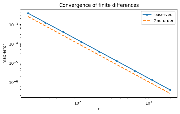
10.5 Nonlinearity and boundary conditions
Example 10.5.2
The first step is to define the function ϕ that equals .
phi = lambda t, theta, omega: -0.05 * omega - sin(theta)Next, we define the boundary conditions.
ga = lambda u, du: u - 2.5
gb = lambda u, du: u + 2
The last ingredient is an initial estimate of the solution. Here we choose and a linear function between the endpoint values.
init = linspace(2.5, -2, 101)We find a solution with negative initial slope, i.e., the pendulum is initially pushed back toward equilibrium.
t, theta = FNC.bvp(phi, [0, 5], ga, gb, init)
plot(t, theta)
xlabel("$t$")
ylabel("$\theta(t)$")
title("Pendulum over [0,5]");
If we extend the time interval longer for the same boundary values, then the initial slope must adjust.
t, theta = FNC.bvp(phi, [0, 8], ga, gb, init)
plot(t, theta)
xlabel("$t$")
ylabel("$\theta(t)$")
title("Pendulum over [0,8]");
This time, the pendulum is initially pushed toward the unstable equilibrium in the upright vertical position before gravity pulls it back down.
Example 10.5.3
Here is the problem definition. We use a truncated domain to avoid division by zero at .
lamb = 0.5
phi = lambda r, w, dwdr: lamb / w**2 - dwdr / r
a, b = finfo(float).eps, 1
ga = lambda w, dw: dw
gb = lambda w, dw: w - 1
First we try a constant function as the initialization.
init = ones(201)
r, w1 = FNC.bvp(phi, [a, b], ga, gb, init)
plot(r, w1)
fig, ax = gcf(), gca()
xlabel("$r$"),  ylabel("$w(r)$")
title("Solution of the MEMS problem");
It’s not necessary that the initialization satisfy the boundary conditions. In fact, by choosing a different constant function as the initial guess, we arrive at another valid solution.
r, w2 = FNC.bvp(phi, [a, b], ga, gb, 0.5 * init)
ax.plot(r, w2)
ax.set_title("Multiple solutions of the MEMS problem");
fig
Example 10.5.4
phi = lambda x, u, dudx: (u**3 - u) / epsilon
ga = lambda u, du: du
gb = lambda u, du: u - 1
Finding a solution is easy at larger values of ε.
epsilon = 0.05
init = linspace(-1, 1, 141)
x, u1 = FNC.bvp(phi, [0, 1], ga, gb, init)

plot(x, u1, label="$\\epsilon = 0.05$")
fig, ax = gcf(), gca()
xlabel("$x$"),  ylabel("$u(x)$")
legend(),  title("Allen-Cahn solution");
Finding a good initialization is not trivial for smaller values of ε. But the iteration succeeds if we use the first solution as the initialization at the smaller ε.
epsilon = 0.002
x, u2 = FNC.bvp(phi, [0, 1], ga, gb, u1)
ax.plot(x, u2, label="$\\epsilon = 0.002$")
ax.legend()
fig
In this case we can continue further.
ϵ = 0.0005
x, u3 = FNC.bvp(phi, [0, 1], ga, gb, u2)
ax.plot(x, u3, label="$\\epsilon = 0.005$")
ax.legend()
fig
10.6 The Galerkin method
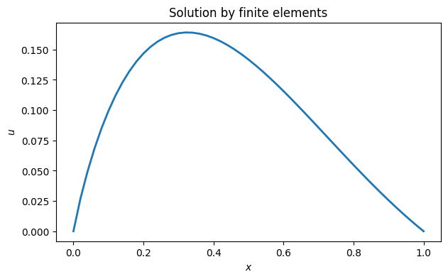
Example 10.6.2
Here are the coefficient function definitions. Even though is a constant, it has to be defined as a function for Function 10.6.1 to use it.
c = lambda x: x**2
q = lambda x: 4 * ones(len(x))
f = lambda x: sin(pi * x)
x, u = FNC.fem(c, q, f, 0, 1, 50)
plot(x, u)
xlabel("$x$"), ylabel("$u$")
title("Solution by finite elements");