Chapter 9 - Fundamentals of Numerical Computation

Functions¶

Barycentric polynomial interpolation

polyinterp.py

1
2
3
4
5
6
7
8
9
10
11
12
13
14
15
16
17
18
19
20
21
22
23
24
25
26
27
28
29
30
31
def polyinterp(t, y):
    """
    polyinterp(t, y)

    Return a callable polynomial interpolant through the points in vectors t, y. Uses
    the barycentric interpolation formula.
    """
    n = len(t) - 1
    C = (t[-1] - t[0]) / 4  # scaling factor to ensure stability
    tc = t / C

    # Adding one node at a time, compute inverses of the weights.
    omega = np.ones(n + 1)
    for m in range(n):
        d = tc[: m + 1] - tc[m + 1]  # vector of node differences
        omega[: m + 1] = omega[: m + 1] * d  # update previous
        omega[m + 1] = np.prod(-d)  # compute the new one
    w = 1 / omega  # go from inverses to weights

    def p(x):
        # Compute interpolant.
        z = np.where(x == t)[0]
        if len(z) > 0:  # avoid dividing by zero
            # Apply L'Hopital's Rule exactly.
            f = y[z[0]]
        else:
            terms = w / (x - t)
            f = np.sum(y * terms) / np.sum(terms)
        return f

    return np.vectorize(p)

Trigonometric interpolation

triginterp.py

1
2
3
4
5
6
7
8
9
10
11
12
13
14
15
16
17
18
19
20
21
def triginterp(t, y):
    """
        triginterp(t, y)

    Return trigonometric interpolant for points defined by vectors t and y.
    """
    N = len(t)

    def trigcardinal(x):
        if x == 0:
            tau = 1.0
        elif np.mod(N, 2) == 1:  # odd
            tau = np.sin(N * np.pi * x / 2) / (N * np.sin(np.pi * x / 2))
        else:  # even
            tau = np.sin(N * np.pi * x / 2) / (N * np.tan(np.pi * x / 2))
        return tau

    def p(x):
        return np.sum([y[k] * trigcardinal(x - t[k]) for k in range(N)])

    return np.vectorize(p)

Clenshaw–Curtis integration

ccint.py

1
2
3
4
5
6
7
8
9
10
11
12
13
14
15
16
17
18
19
20
21
22
23
def ccint(f, n):
    """
    ccint(f, n)

    Perform Clenshaw-Curtis integration for the function f on n+1 nodes in [-1,1]. Return
    integral and a vector of the nodes used. Note: n must be even.
    """
    # Find Chebyshev extreme nodes.
    theta = np.linspace(0, np.pi, n + 1)
    x = -np.cos(theta)

    # Compute the C-C weights.
    c = np.zeros(n + 1)
    c[[0, n]] = 1 / (n**2 - 1)
    v = np.ones(n - 1)
    for k in range(1, int(n / 2)):
        v -= 2 * np.cos(2 * k * theta[1:-1]) / (4 * k**2 - 1)
    v -= np.cos(n * theta[1:-1]) / (n**2 - 1)
    c[1:-1] = 2 * v / n

    # Evaluate integrand and integral.
    I = np.dot(c, f(x))  # use vector inner product
    return I, x

Gauss–Legendre integration

glint.py

1
2
3
4
5
6
7
8
9
10
11
12
13
14
15
16
17
18
19
def glint(f, n):
    """
    glint(f, n)

    Perform Gauss-Legendre integration for the function f on n nodes in (-1,1). Return
    integral and a vector of the nodes used.
    """
    # Nodes and weights are found via a tridiagonal eigenvalue problem.
    beta = 0.5 / np.sqrt(1 - (2.0 * np.arange(1, n)) ** (-2))
    T = np.diag(beta, 1) + np.diag(beta, -1)
    ev, V = eig(T)
    ev = np.real_if_close(ev)
    p = np.argsort(ev)
    x = ev[p]  # nodes
    c = 2 * V[0, p] ** 2  # weights

    # Evaluate the integrand and compute the integral.
    I = np.dot(c, f(x))  # vector inner product
    return I, x

Integration over

(-\infty,\infty)

intinf.py

1
2
3
4
5
6
7
8
9
10
11
12
13
14
15
16
17
18
19
20
21
def intinf(f, tol):
    """
    intinf(f, tol)

    Perform doubly-exponential integration of function f over (-Inf,Inf), using
    error tolerance tol. Return integral and a vector of the nodes used.
    """
    xi = lambda t: np.sinh(np.sinh(t))
    dxi_dt = lambda t: np.cosh(t) * np.cosh(np.sinh(t))
    g = lambda t: f(xi(t)) * dxi_dt(t)
    M = 3
    while (abs(g(-M)) > tol/100) or (abs(g(M)) > tol/100):
        M += 0.5
        if np.isinf(xi(M)):
            warnings.warn("Function may not decay fast enough.")
            M -= 0.5
            break

    I, t = intadapt(g,-M,M,tol)
    x = xi(t)
    return I, x

Integration with endpoint singularities

intsing.py

1
2
3
4
5
6
7
8
9
10
11
12
13
14
15
16
17
18
19
20
21
22
23
def intsing(f, tol):
    """
    intsing(f, tol)

    Adaptively integrate function f over (0,1), where f may be 
    singular at zero, with error tolerance tol. Returns the
    integral estimate and a vector of the nodes used.
    """
    xi = lambda t: 2 / (1 + np.exp( 2*np.sinh(t) ))
    dxi_dt = lambda t: np.cosh(t) / np.cosh(np.sinh(t))**2
    g = lambda t: f(xi(t)) * dxi_dt(t)
    # Find where to truncate the integration interval.
    M = 3
    while abs(g(M)) > tol/100:
        M += 0.5
        if xi(M) == 0:
            warnings.warn("Function may grow too rapidly.")
            M -= 0.5
            break

    I, t = intadapt(g, 0, M, tol)
    x = xi(t)
    return I, x

Examples¶

9.1 Polynomial interpolation¶

Example 9.1.1

Here is a vector of nodes.

t = array([1, 1.5, 2, 2.25, 2.75, 3])
n = 5

Let’s apply the definition of the cardinal Lagrange polynomial for $k=2$ . First we define a polynomial $q$ that is zero at all the nodes except $i=k$ . Then $\ell_2$ is found by normalizing $q$ by $q(t_k)$ .

k = 2
q = lambda x: prod([x - t[i] for i in range(n + 1) if i != k])
ell_k = lambda x: q(x) / q(t[k])

A plot confirms the cardinal property of the result.

x = linspace(1, 3, 500)
plot(x, [ell_k(xx) for xx in x])
y = zeros(n+1)
y[k] = 1
plot(t, y, "ko")
xlabel("$x$"),  ylabel("$\\ell_2(x)$")
title(("Lagrange cardinal function"));

Observe that $\ell_k$ is not between zero and one everywhere, unlike a hat function.

Example 9.1.3

from scipy.interpolate import BarycentricInterpolator as interp
t = array([1, 1.6, 1.9, 2.7, 3])
p = interp(t, log(t))

from scipy.interpolate import BarycentricInterpolator as interp
t = array([1, 1.6, 1.9, 2.7, 3])
p = interp(t, log(t))
x = linspace(1, 3, 500)
Phi = lambda x: prod([x - ti for ti in t])
plot(x, [Phi(xj) / 5 for xj in x], label="$\\frac{1}{5}|\\Phi(x)|$")
plot(x, abs(log(x) - p(x)), label="$|f(x)-p(x)|$")
plot(t, zeros(t.size), "ko", label="nodes")
xlabel("$x$"),  ylabel("error")
title("Interpolation error and upper bound"),  legend();

The error is zero at the nodes, by the definition of interpolation. The error bound, as well as the error itself, has one local maximum between each consecutive pair of nodes.

9.2 The barycentric formula¶

Example 9.2.2

f = lambda x: sin(exp(2 * x))
x = linspace(0, 1, 500)
fig, ax = subplots()
ax.plot(x, f(x), label="function")

t = linspace(0, 1, 4)
y = f(t)
p = FNC.polyinterp(t, y)

ax.plot(x, p(x), label="interpolant")
ax.plot(t, y, "ko", label="nodes")
ax.legend()
ax.set_title("Interpolation on 4 nodes")
fig

The curves must intersect at the interpolation nodes. For $n=6$ the interpolant is noticeably better.

plot(x, f(x), label="function")
t = linspace(0, 1, 7)
y = f(t)
p = FNC.polyinterp(t, y)
plot(x, p(x), label="interpolant")
plot(t, y, "ko", label="nodes")
legend(),  title("Interpolation on 7 nodes");

9.3 Stability of polynomial interpolation¶

Example 9.3.1

We choose a function over the interval $[0,1]$ .

f = lambda x: sin(exp(2 * x))

Here is a graph of $f$ and its polynomial interpolant using seven equally spaced nodes.

x = linspace(0, 1, 500)
plot(x, f(x), label="function")
t = linspace(0, 1, 7)
y = f(t)
p = FNC.polyinterp(t, y)
plot(x, p(x), label="interpolant")
plot(t, y, 'ko', label="nodes")
legend(),  title("Equispaced interpolant, n=6");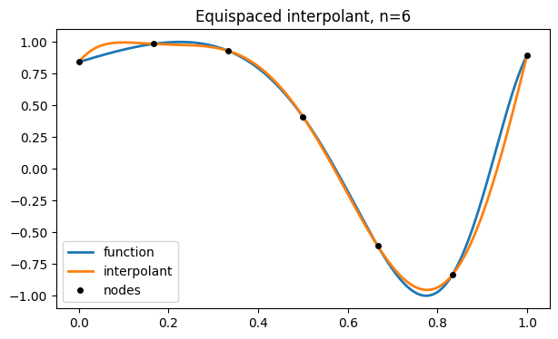

This looks pretty good. We want to track the behavior of the error as $n$ increases. We will estimate the error in the continuous interpolant by sampling it at a large number of points and taking the max-norm.

N = arange(5, 65, 5)
err = zeros(N.size)
x = linspace(0, 1, 1001)         # for measuring error
for k, n in enumerate(N):
    t = linspace(0, 1, n + 1)    # equally spaced nodes
    y = f(t)  # interpolation data
    p = FNC.polyinterp(t, y)
    err[k] = max(abs(f(x) - p(x)))

semilogy(N, err, "-o")
xlabel("$n$"),  ylabel("max error")
title(("Polynomial interpolation error"));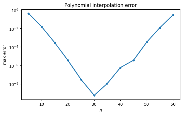

The error initially decreases as one would expect but then begins to grow. Both phases occur at rates that are exponential in $n$ , i.e., $O(K^n$ ) for a constant $K$ , appearing linear on a semi-log plot.

Example 9.3.2

We plot $|\Phi(x)|$ over the interval $[-1,1]$ with equispaced nodes for different values of $n$ .

x = linspace(-1, 1, 1601)
for n in range(10, 60, 10):
    t = linspace(-1, 1, n + 1)
    Phi = array([prod(xk - t) for xk in x])
    semilogy(x, abs(Phi), ".", markersize=2)
xlabel("$x$")
ylabel("$|\Phi(x)|$")
ylim([1e-25, 1])
title(("Effect of equispaced nodes"));

<>:7: SyntaxWarning: invalid escape sequence '\P'
<>:7: SyntaxWarning: invalid escape sequence '\P'
/var/folders/gc/0752xrm56pnf0r0dsrn5370c0000gr/T/ipykernel_93667/3615654825.py:7: SyntaxWarning: invalid escape sequence '\P'
  ylabel("$|\Phi(x)|$")

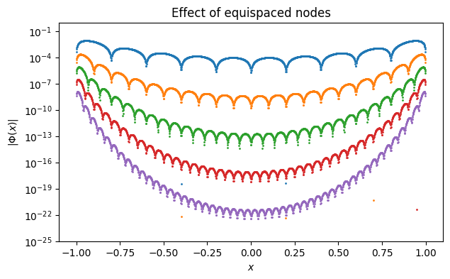
Each time Φ passes through zero at an interpolation node, the value on the log scale should go to $-\infty$ , which explains the numerous cusps on the curves.

Example 9.3.3

This function has infinitely many continuous derivatives on the entire real line and looks easy to approximate over $[-1,1]$ .

f = lambda x: 1 / (x**2 + 16)
x = linspace(-1, 1, 1601)
plot(x, f(x))
title("Test function");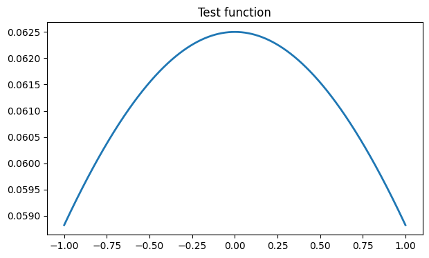

We start by doing equispaced polynomial interpolation for some small values of $n$ .

N = arange(4, 16, 4)
label = []
for k, n in enumerate(N):
    t = linspace(-1, 1, n + 1)  # equally spaced nodes
    y = f(t)  # interpolation data
    p = FNC.polyinterp(t, y)
    err = abs(f(x) - p(x))
    semilogy(x, err, ".", markersize=2)
    label.append(f"degree {n}")

xlabel("$x$"),  ylabel("$|f(x)-p(x)|$")
ylim([1e-20, 1])
legend(label),  title("Error for low degrees");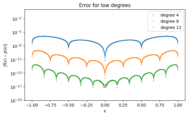

The convergence so far appears rather good, though not uniformly so. However, notice what happens as we continue to increase the degree.

N = 12 + 15 * arange(1, 4)
labels = []
for k, n in enumerate(N):
    t = linspace(-1, 1, n + 1)  # equally spaced nodes
    y = f(t)  # interpolation data
    p = FNC.polyinterp(t, y)
    err = abs(f(x) - p(x))
    semilogy(x, err, ".", markersize=2)
    labels.append(f"degree {n}")
xlabel("$x$"),  ylabel("$|f(x)-p(x)|$"),  ylim([1e-20, 1])
legend(labels),  title("Error for higher degrees");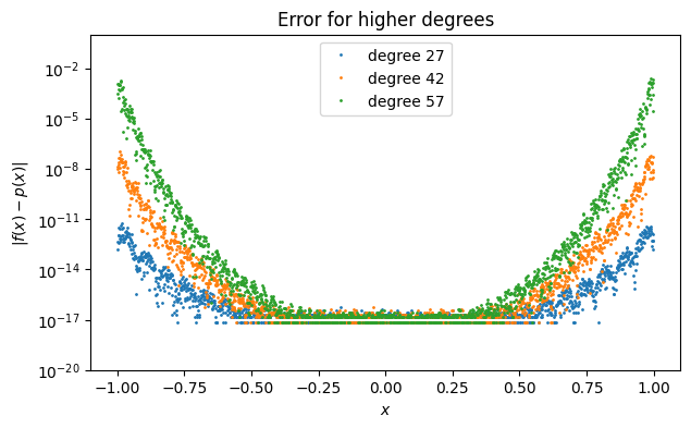

The convergence in the middle can’t get any better than machine precision relative to the function values. So maintaining the growing gap between the center and the ends pushes the error curves upward exponentially fast at the ends, wrecking the convergence.

Example 9.3.4

Now we look at the error indicator function Φ for Chebyshev node sets.

x = linspace(-1, 1, 1601)
labels = []
for n in range(10, 60, 10):
    theta = pi * arange(n + 1) / n
    t = -cos(theta)
    Phi = array([prod(xk - t) for xk in x])
    semilogy(x, abs(Phi), ".")
    labels.append(f"degree {n}")

xlabel("$x$"),  ylabel("$|\\Phi(x)|$"),  ylim([1e-18, 1e-2])
legend(labels),  title("Error indicator for Chebyshev nodes");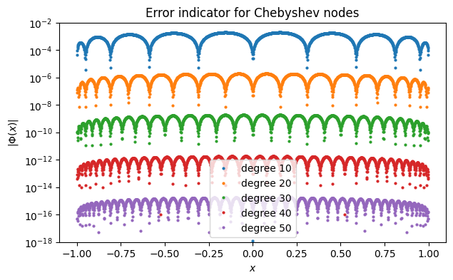

In contrast to the equispaced case, $|\Phi|$ decreases exponentially with $n$ almost uniformly across the interval.

Example 9.3.5

Here again is the function from Demo 9.3.3 that provoked the Runge phenomenon when using equispaced nodes.

f = lambda x: 1 / (x**2 + 16)

x = linspace(-1, 1, 1601)
labels = []
for k, n in enumerate([4, 10, 16, 40]):
    t = -cos(pi * arange(n + 1) / n)         # Chebyshev nodes
    y = f(t)                                 # interpolation data
    p = FNC.polyinterp(t, y)
    err = abs(f(x) - p(x))
    semilogy(x, err, ".", markersize=2)
    labels.append(f"degree {n}")

xlabel("$x$"),  ylabel("$|f(x)-p(x)|$"),  ylim([1e-20, 1])
legend(labels),  title("Error for Chebyshev interpolants");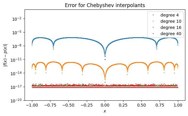

By degree 16 the error is uniformly within machine epsilon, and, importantly, it stays there as $n$ increases. Note that as predicted by the error indicator function, the error is uniform over the interval at each value of $n$ .

Example 9.3.6

On the left, we use a log-log scale, which makes second-order algebraic convergence $O(n^{-4})$ a straight line. On the right, we use a log-linear scale, which makes spectral convergence $O(K^{-n})$ linear.

n = arange(20, 420, 20)
algebraic = 100 / n**4
spectral = 10 * 0.85**n

subplot(2, 1, 1)
loglog(n, algebraic, 'o-', label="algebraic")
loglog(n, spectral, 'o-', label="spectral")
xlabel('n'),  ylabel('error') 
title('log–log'), ylim([1e-16, 1]);
legend() 

subplot(2, 1, 2)
semilogy(n, algebraic, 'o-', label="algebraic")
semilogy(n, spectral, 'o-', label="spectral")
xlabel('n'),  ylabel('error')
title('log–linear') ,  ylim([1e-16, 1]);  
legend();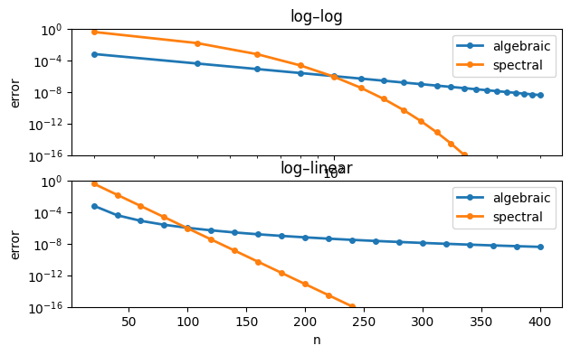

9.4 Orthogonal polynomials¶

Example 9.4.1

Let’s approximate $e^x$ over the interval $[−1,1]$ . We can sample it at, say, 15 points, and find the best-fitting straight line to that data.

from numpy.linalg import lstsq
t = linspace(-1, 1, 15)
y = exp(t)
plot(t, y, label="function")

V = [[ti**j for j in range(2)] for ti in t]
c = lstsq(V, y, rcond=None)[0]
print("fit coeffs:", c)

x = linspace(-1, 1, 600)
plot(x, c[1] + c[0] * x, label="fit")
xlabel("x"),  ylabel("value")
legend(),  title("Least squares fit of exp(x)");

fit coeffs: [1.20159125 1.11828384]

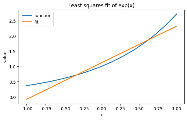
There’s nothing special about 15 points. Choosing more doesn’t change the result much.

t = linspace(-1, 1, 150)
y = exp(t)
plot(t, y, label="function")

V = [[ti**j for j in range(2)] for ti in t]
c = lstsq(V, y, rcond=None)[0]
print("fit coeffs:", c)

x = linspace(-1, 1, 600)
plot(x, c[1] + c[0] * x, label="fit")
xlabel("x"),  ylabel("value")
legend(),  title("Least squares fit of exp(x)");

fit coeffs: [1.17767125 1.10507318]

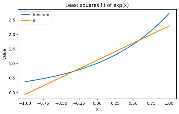
This situation is unlike interpolation, where the degree of the interpolant increases with the number of nodes. Here, the linear fit is apparently approaching a limit that we may think of as a continuous least-squares fit.

n = arange(40, 420, 60)
results = PrettyTable(["n", "intercept", "slope"])
slope = zeros(n.size)
intercept = zeros(n.size)

for k in range(n.size):
    t = linspace(-1, 1, n[k])
    y = exp(t)
    V = [[ti**j for j in range(2)] for ti in t]
    c = lstsq(V, y, rcond=None)[0]
    results.add_row([n[k], c[1], c[0]])

print(results)

+-----+--------------------+--------------------+
|  n  |     intercept      |       slope        |
+-----+--------------------+--------------------+
|  40 | 1.1090551764670025 | 1.1846492800335242 |
| 100 | 1.105793288180965  | 1.1789195568501283 |
| 160 | 1.1049832955976737 | 1.1775158384490085 |
| 220 | 1.1046158595861273 | 1.176881503540092  |
| 280 | 1.1044061059639807 | 1.1765200632992356 |
| 340 | 1.1042704646318244 | 1.1762865906944795 |
| 400 | 1.1041755539295632 | 1.1761233467177028 |
+-----+--------------------+--------------------+

9.5 Trigonometric interpolation¶

Example 9.5.1

We will get a cardinal function without using an explicit formula, just by passing data that is 1 at one node and 0 at the others.

N = 7
n = int((N - 1) / 2)
t = 2 * arange(-n, n + 1) / N
y = zeros(N)
y[n] = 1

p = FNC.triginterp(t, y)
x = linspace(-1, 1, 600)
plot(x, p(x))
plot(t, y, "ko")

xlabel("x"),  ylabel("tau(x)")
title("Trig cardinal function");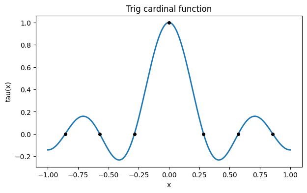

Here is a 2-periodic function and one of its interpolants.

f = lambda x: exp(sin(pi * x) - 2 * cos(pi * x))

plot(x, f(x), label="periodic function")
y = f(t)

p = FNC.triginterp(t, y)
plot(x, p(x), label="trig interpolant")
plot(t, y, "ko", label="nodes")

xlabel("$x$"),  ylabel("$p(x)$")
legend(),  title("Trig interpolation");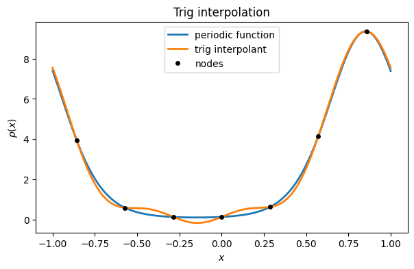

The convergence of the interpolant is spectral. We let $N$ go needlessly large here in order to demonstrate that unlike polynomials, trigonometric interpolation is stable on equally spaced nodes. Note that when $N$ is even, the value of $n$ is not an integer but works fine for defining the nodes.

N = arange(2, 62, 2)
err = zeros(N.size)

x = linspace(-1, 1, 1601)    # for measuring error
for k in range(N.size):
    n = (N[k] - 1) / 2
    t = 2 * arange(-n, n + 1) / N[k]
    p = FNC.triginterp(t, f(t))
    err[k] = max(abs(f(x) - p(x)))

semilogy(N, err, "-o")
xlabel("N"),  ylabel("max error")
title("Convergence of trig interpolation");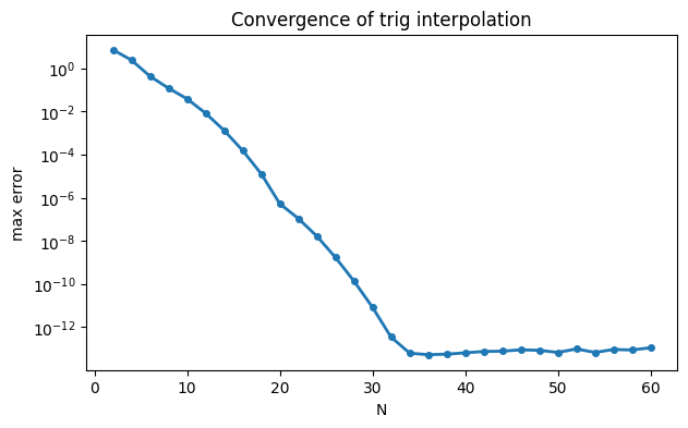

Example 9.5.2

This function has frequency content at $2\pi$ , $-2\pi$ , and π.

f = lambda x: 3 * cos(2 * pi * x) - exp(1j * pi * x)

To use fft, we set up nodes in the interval $[0,2)$ .

n = 4
N = 2 * n + 1
t = 2 * arange(0, N) / N    # nodes in [0,2)
y = f(t)

We perform Fourier analysis using fft and then examine the resulting coefficients.

from scipy.fftpack import fft, ifft, fftshift
c = fft(y) / N
freq = hstack([arange(n+1), arange(-n,0)])
results = PrettyTable()
results.add_column("freq", freq) 
results.add_column("coefficient", c)
results

Note that $1.5 e^{2i\pi x}+1.5 e^{-2i\pi x} = 3 \cos(2\pi x)$ , so this result is sensible.

Fourier’s greatest contribution to mathematics was to point out that every periodic function is just a combination of frequencies—infinitely many of them in general, but truncated for computational use. Here we look at the magnitudes of the coefficients for $f(x) = \exp( \sin(\pi x) )$ .

f = lambda x: exp(sin(pi * x))    # content at all frequencies
n = 9;  N = 2*n + 1;
t = 2 * arange(0, N) / N    # nodes in [0,2)
c = fft(f(t)) / N

semilogy(range(-n, n+1), abs(fftshift(c)), "o")
xlabel("$k$"),  ylabel("$|c_k|$")
title("Fourier coefficients");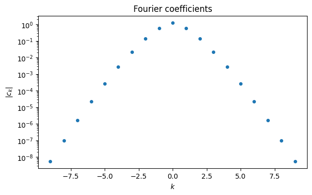

The Fourier coefficients of smooth functions decay exponentially in magnitude as a function of the frequency. This decay rate is determines the convergence of the interpolation error.

9.6 Spectrally accurate integration¶

Example 9.6.1

f = lambda t: pi * sqrt(cos(pi * t) ** 2 + sin(pi * t) ** 2 / 4)
N = arange(4, 48, 6)
perim = zeros(N.size)
for k in range(N.size):
    h = 2 / N[k]
    t = h * arange(N[k]) - 1
    perim[k] = h * sum(f(t))
err = abs(perim - perim[-1])    # use the last value as reference
results = PrettyTable()
results.add_column("N", N)
results.add_column("perimeter", perim)
results.add_column("error", err)
results

The approximations gain about one digit of accuracy for each constant increment of $n$ , which is consistent with spectral convergence.

Example 9.6.3

First consider the integral

\int_{-1}^1 \frac{1}{1+4x^2} \, dx = \arctan(2).

(1)

f = lambda x: 1 / (1 + 4 * x**2)
exact = arctan(2)

We compare the two spectral integration methods for a range of $n$ values.

N = range(8, 100, 4)
errCC = zeros(len(N))
errGL = zeros(len(N))
for k, n in enumerate(N):
    errCC[k] = exact - FNC.ccint(f, n)[0]
    errGL[k] = exact - FNC.glint(f, n)[0]

semilogy(N, abs(errCC), "-o", label="Clenshaw–Curtis")
semilogy(N, abs(errGL), "-o", label="Gauss–Legendre")
xlabel("number of nodes"),  ylabel("error"),  ylim(1e-16, 0.01)
legend(),  title("Spectral integration");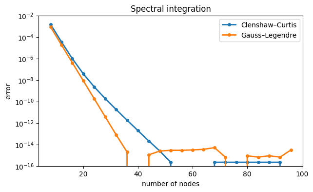

(The missing dots are where the error is exactly zero.) Gauss–Legendre does converge faster here, but at something less than twice the rate.

Now we try a more sharply peaked integrand:

\int_{-1}^1 \frac{1}{1+16x^2} \, dx = \frac{1}{2}\arctan(4).

(2)

f = lambda x: 1 / (1 + 16 * x**2)
exact = atan(4) / 2

N = range(8, 100, 4)
errCC = zeros(len(N))
errGL = zeros(len(N))
for k, n in enumerate(N):
    errCC[k] = exact - FNC.ccint(f, n)[0]
    errGL[k] = exact - FNC.glint(f, n)[0]

semilogy(N, abs(errCC), "-o", label="Clenshaw–Curtis")
semilogy(N, abs(errGL), "-o", label="Gauss–Legendre")
xlabel("number of nodes"),  ylabel("error"),  ylim(1e-16, 0.1)
legend(),  title("Spectral integration");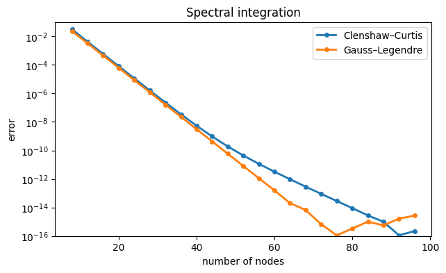

The two are very close until about $n=40$ , when the Clenshaw–Curtis method slows down.

Now let’s compare the spectral performance to that of our earlier adaptive method in intadapt. We will specify varying error tolerances and record the error as well as the total number of evaluations of $f$ .

loglog(N, abs(errCC), "-o", label="ccint")
loglog(N, abs(errGL), "-o", label="glint")

tol_ = 1 / 10 ** arange(2, 15)
n = zeros(tol_.size)
errAdapt = zeros(tol_.size)
for k, tol in enumerate(tol_):
    Q, t = FNC.intadapt(f, -1, 1, tol)
    errAdapt[k] = exact - Q
    n[k] = t.size

loglog(n, abs(errAdapt), "-o", label="intadapt")
loglog(n, 1 / (n**4), "--", label="4th order")
xlabel("number of nodes"),  ylabel("error"),  ylim(1e-16, 1)
legend(),  title("Spectral vs 4th order");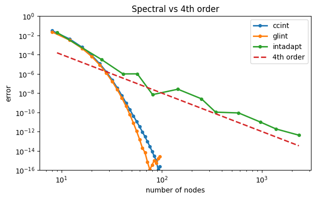

At the core of intadapt is a fourth-order formula, and the results track that rate closely. For all but the most relaxed error tolerances, both spectral methods are far more efficient than the low-order counterpart. For other integrands, particularly those that vary nonuniformly across the interval, the adaptive method might be more competitive.

9.7 Improper integrals¶

Example 9.7.2

f = lambda x: 1 / (1 + x**2)
x = linspace(-4, 4, 500)
subplot(2, 1, 1)
plot(x, f(x)),  yscale('log')
xlabel('x'),  ylabel('f(x)'),  ylim([1e-16, 1])  
title('Original integrand')   

xi = lambda t: sinh( pi * sinh(t) / 2 )
dxi_dt = lambda t: pi/2 * cosh(t) * cosh( pi * sinh(t) / 2 )
integrand = lambda t: f(xi(t)) * dxi_dt(t)
subplot(2, 1, 2)
plot(x, integrand(x)),  yscale('log')
xlabel('t'),  ylabel('f(x(t))'),  ylim([1e-16, 1])  
title('Transformed integrand')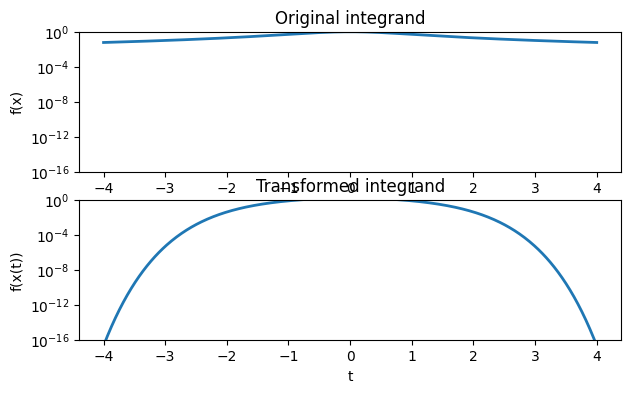

This graph suggests that we capture all of the integrand values that are larger than machine epsilon by integrating in $t$ from -4 to 4.

Example 9.7.3

f = lambda x: 1 / (1 + x**2)
exact = pi
tol = array([1 / 10**d for d in arange(5, 14, 0.5)])
err = zeros((tol.size, 2))
length = zeros((tol.size, 2))
for k in range(tol.size):
    I1, x1 = FNC.intadapt(f, -2/tol[k], 2/tol[k], tol[k])
    I2, x2 = FNC.intinf(f, tol[k])
    err[k] = abs(exact - array([I1, I2]))
    length[k] = [x1.size, x2.size]
loglog(length, err, "-o")
# plot(len,err,m=:o,label=["direct" "double exponential"])
n = array([100, 10000])
loglog(n, 1000 / n**4, 'k--')
xlabel("number of nodes"),  ylabel("error")
title("Comparison of integration methods")
legend(["direct", "double exponential", "4th-order"], loc="lower left");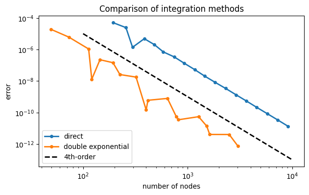

Both methods are roughly fourth-order due to Simpson’s formula in the underlying adaptive integration method. At equal numbers of evaluation nodes, however, the double exponential method is consistently 2--3 orders of magnitude more accurate.

Example 9.7.4

f = lambda x: 1 / (10 * sqrt(x))
exact = 0.2
tol = array([1 / 10**d for d in arange(5, 14, 0.5)])
err = zeros((tol.size, 2))
length = zeros((tol.size, 2))
for k in range(tol.size):
    I1, x1 = FNC.intadapt(f, (tol[k]/20)**2, 1, tol[k])
    I2, x2 = FNC.intsing(f, tol[k])
    err[k] = abs(exact - array([I1, I2]))
    length[k] = [x1.size, x2.size]
loglog(length, err, "-o")
# plot(len,err,m=:o,label=["direct" "double exponential"])
n = array([100, 10000])
loglog(n, 30 / n**4, 'k--')
xlabel("number of nodes"),  ylabel("error")
title("Comparison of integration methods")
legend(["direct", "double exponential", "4th-order"], loc="lower left");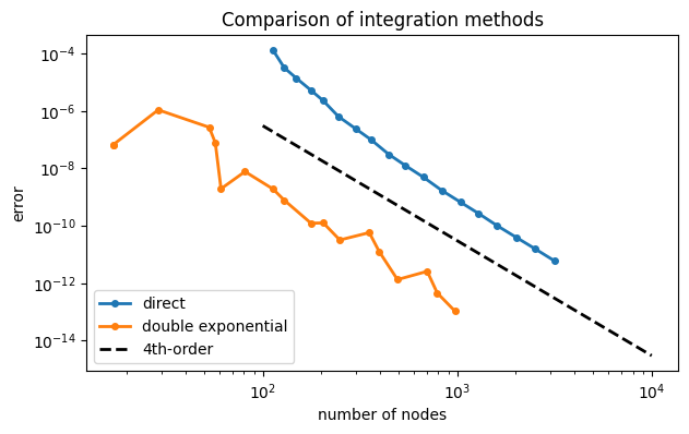

As in Demo 9.7.3, the double exponential method is more accurate than direct integration by a few orders of magnitude. Equivalently, the same accuracy can be reached with many fewer nodes.