Chapter 8 - Fundamentals of Numerical Computation

Functions¶

Power iteration

poweriter.py

1
2
3
4
5
6
7
8
9
10
11
12
13
14
15
16
17
18
def poweriter(A, numiter):
    """
    poweriter(A, numiter)

    Perform numiter power iterations with the matrix A, starting from a random vector, 
    and return a vector of eigenvalue estimates and the final eigenvector approximation.
    """
    n = A.shape[0]
    x = np.random.randn(n)
    x = x / np.linalg.norm(x, np.inf)
    gamma = np.zeros(numiter)
    for k in range(numiter):
        y = A @ x
        m = np.argmax(abs(y))
        gamma[k] = y[m] / x[m]
        x = y / y[m]

    return gamma, x

Inverse iteration

inviter.py

1
2
3
4
5
6
7
8
9
10
11
12
13
14
15
16
17
18
19
20
def inviter(A, s, numiter):
    """
    inviter(A, s, numiter)

    Perform numiter inverse iterations with the matrix A and shift s, starting
    from a random vector, and return a vector of eigenvalue estimates and the final
    eigenvector approximation.
    """
    n = A.shape[0]
    x = np.random.randn(n)
    x = x / np.linalg.norm(x, np.inf)
    gamma = np.zeros(numiter)
    PL, U = lu(A - s * np.eye(n), permute_l=True)
    for k in range(numiter):
        y = np.linalg.solve(U, np.linalg.solve(PL, x))
        m = np.argmax(abs(y))
        gamma[k] = x[m] / y[m] + s
        x = y / y[m]

    return gamma, x

Arnoldi iteration

arnoldi.py

1
2
3
4
5
6
7
8
9
10
11
12
13
14
15
16
17
18
19
20
21
22
23
24
def arnoldi(A, u, m):
    """
    arnoldi(A, u, m)

    Perform the Arnoldi iteration for A starting with vector u, out to the Krylov
    subspace of degree m. Return the orthonormal basis (m+1 columns) and the upper
    Hessenberg H of size m+1 by m.
    """
    n = u.size
    Q = np.zeros([n, m + 1])
    H = np.zeros([m + 1, m])
    Q[:, 0] = u / np.linalg.norm(u)
    for j in range(m):
        # Find the new direction that extends the Krylov subspace.
        v = A @ Q[:, j]
        # Remove the projections onto the previous vectors.
        for i in range(j + 1):
            H[i, j] = Q[:, i] @ v
            v -= H[i, j] * Q[:, i]
        # Normalize and store the new basis vector.
        H[j + 1, j] = np.linalg.norm(v)
        Q[:, j + 1] = v / H[j + 1, j]

    return Q, H

GMRES

gmres.py

1
2
3
4
5
6
7
8
9
10
11
12
13
14
15
16
17
18
19
20
21
22
23
24
25
26
27
28
29
30
31
32
def gmres(A, b, m):
    """
    gmres(A, b, m)

    Do m iterations of GMRES for the linear system A*x=b. Return the final solution
    estimate x and a vector with the history of residual norms. (This function is for
    demo only, not practical use.)
    """
    n = len(b)
    Q = np.zeros([n, m + 1])
    Q[:, 0] = b / np.linalg.norm(b)
    H = np.zeros([m + 1, m])

    # Initial "solution" is zero.
    residual = np.hstack([np.linalg.norm(b), np.zeros(m)])

    for j in range(m):
        # Next step of Arnoldi iteration.
        v = A @ Q[:, j]
        for i in range(j + 1):
            H[i, j] = Q[:, i] @ v
            v -= H[i, j] * Q[:, i]
        H[j + 1, j] = np.linalg.norm(v)
        Q[:, j + 1] = v / H[j + 1, j]

        # Solve the minimum residual problem.
        r = np.hstack([np.linalg.norm(b), np.zeros(j + 1)])
        z = np.linalg.lstsq(H[:j + 2, :j + 1], r)[0]
        x = Q[:, :j + 1] @ z
        residual[j + 1] = np.linalg.norm(A @ x - b)

    return x, residual

Examples¶

8.1 Sparsity and structure¶

Example 8.1.1

Here we load the adjacency matrix of a graph with 2790 nodes. Each node is a web page referring to Roswell, NM, and the edges represent links between web pages. (Credit goes to Panayiotis Tsaparas and the University of Toronto for making this data public.)

import scipy.sparse as sp
from scipy.io import loadmat

vars = loadmat("roswelladj.mat")    # get from the book's website
A = sp.csr_matrix(vars["A"])

We may define the density of $\mathbf{A}$ as the number of nonzeros divided by the total number of entries.

m, n = A.shape
print(f"density is {A.nnz / (m * n):.3%}")

density is 0.109%

We can compare the storage space needed for the sparse $\mathbf{A}$ with the space needed for its dense / full counterpart.

F = A.todense()
print(f"{A.data.nbytes/1e6:.3f} MB for sparse form, {F.nbytes/1e6:.3f} MB for dense form")

0.068 MB for sparse form, 62.273 MB for dense form

Matrix-vector products are also much faster using the sparse form because operations with structural zeros are skipped.

from timeit import default_timer as timer
x = random.randn(n)
start = timer()
for i in range(1000):
    A @ x
print(f"sparse time: {timer() - start:.4g} sec")

sparse time: 0.01756 sec

start = timer()
for i in range(1000):
    F @ x
print(f"dense time: {timer() - start:.4g} sec")

dense time: 14.12 sec

Example 8.1.2

Here is the adjacency matrix of a graph representing a small-world network, featuring connections to neighbors and a small number of distant contacts.

import networkx as nx
wsg = nx.watts_strogatz_graph(200, 4, 0.02)

Because each node connects to relatively few others, the adjacency matrix is quite sparse.

A = nx.adjacency_matrix(wsg)
spy(A)
title("Adjacency matrix $A$");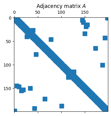

By Theorem 7.1.1, the entries of $\mathbf{A}^k$ give the number of walks of length $k$ between pairs of nodes, as with “k degrees of separation” within a social network. As $k$ grows, the density of $\mathbf{A}^k$ also grows.

from scipy.sparse.linalg import matrix_power
spy(matrix_power(A, 6))
title(("$A^6$"));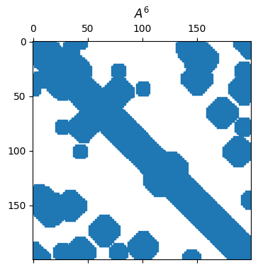

Example 8.1.3

The scipi.sparse.diags function creates a sparse matrix given its diagonal elements and the diagonal indexes to put them on. The main or central diagonal is numbered zero, above and to the right of that is positive, and below and to the left is negative.

n = 50
data = [n * ones(n-3), ones(n), linspace(-1, 1-n, n-1)]
offsets = [-3, 0, 1]    # 3rd below, main, 1st above
A = sp.diags(data, offsets, format="lil")
print(A[:7, :7].todense())

[[ 1. -1.  0.  0.  0.  0.  0.]
 [ 0.  1. -2.  0.  0.  0.  0.]
 [ 0.  0.  1. -3.  0.  0.  0.]
 [50.  0.  0.  1. -4.  0.  0.]
 [ 0. 50.  0.  0.  1. -5.  0.]
 [ 0.  0. 50.  0.  0.  1. -6.]
 [ 0.  0.  0. 50.  0.  0.  1.]]

Without pivoting, the LU factors have the same lower and upper bandwidth as the original matrix.

L, U = FNC.lufact(A.todense())
subplot(1, 2, 1), spy(L)
subplot(1, 2, 2), spy(U);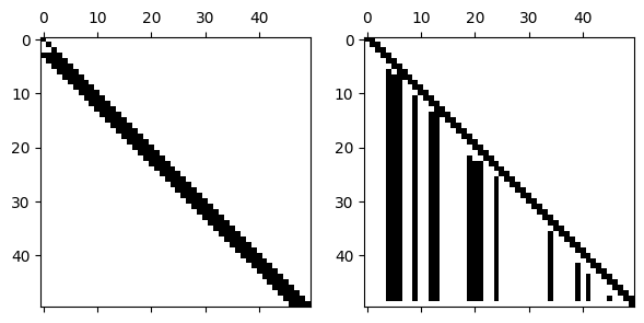

However, if we introduce row pivoting, bandedness may be expanded or destroyed.

L, U, p = FNC.plufact(A.todense())
subplot(1, 2, 1), spy(L[p, :])
subplot(1, 2, 2), spy(U)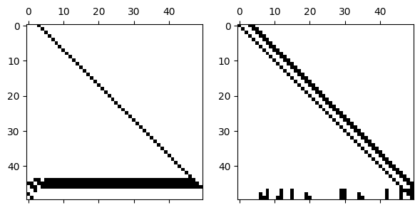

Example 8.1.4

The following generates a random sparse matrix with prescribed eigenvalues.

n = 4000
density = 4e-4
ev = 1 / arange(1, n + 1)
A = FNC.sprandsym(n, density, eigvals=ev)
print(f"density is {A.nnz / prod(A.shape):.3%}")

density is 0.040%

The eigs function finds a small number eigenvalues meeting some criterion. First, we ask for the 5 of largest (complex) magnitude using which="LM".

from scipy.sparse.linalg import eigs
ev, V = eigs(A, k=5, which="LM")    # largest magnitude
print(1 / ev)

[1.+0.j 2.+0.j 3.+0.j 4.+0.j 5.+0.j]

Now we find the 4 closest to the value 1 in the complex plane, via sigma=1.

from scipy.sparse.linalg import eigs
ev, V = eigs(A, k=4, sigma=0.03)    # closest to sigma
print(ev)

[0.03030303+0.j 0.02941176+0.j 0.03125   +0.j 0.02857143+0.j]

The time needed to solve a sparse linear system is not easy to predict unless you have some more information about the matrix. But it will typically be orders of magnitude faster than the dense version of the same problem.

from scipy.sparse.linalg import spsolve
x = 1 / arange(1, n + 1)
b = A @ x
start = timer()
xx = spsolve(A, b)
print(f"sparse time: {timer() - start:.3g} sec")
print(f"residual: {norm(b - A @ xx, 2):.1e}")

sparse time: 0.0015 sec
residual: 5.3e-18

from numpy.linalg import solve
F = A.todense()
start = timer()
xx = solve(F, b)
print(f"dense time: {timer() - start:.3g} sec")
print(f"residual: {norm(b - A @ xx, 2):.1e}")

dense time: 0.665 sec
residual: 5.2e-18

8.2 Power iteration¶

Example 8.2.1

Here we choose a random 5×5 matrix and a random 5-vector.

A = random.choice(range(10), (5, 5))
A = A / sum(A, 0)
x = random.randn(5)
print(x)

[ 0.16978275 -1.13985535 -0.10207207  0.70204959 -0.55130676]

Applying matrix-vector multiplication once doesn’t do anything recognizable.

y = A @ x
print(y)

[ 0.04580142 -0.07757707 -0.15931028 -0.61958189 -0.11073401]

Repeating the multiplication still doesn’t do anything obvious.

z = A @ y
print(z)

[-0.12046302 -0.18321533 -0.2097453  -0.10789248 -0.3000857 ]

But if we keep repeating the matrix-vector multiplication, something remarkable happens: $\mathbf{A} \mathbf{x} \approx \mathbf{x}$ .

x = random.randn(5)
for j in range(6):
    x = A @ x
print(x)
print(A @ x)

[-0.06228606 -0.06954688 -0.07498971 -0.08668721 -0.11640553]
[-0.06256514 -0.06945653 -0.07509878 -0.08617613 -0.1166188 ]

This phenomenon is unlikely to be a coincidence!

Example 8.2.2

We will experiment with the power iteration on a 5×5 matrix with prescribed eigenvalues and dominant eigenvalue at 1.

ev = [1, -0.75, 0.6, -0.4, 0]
A = triu(ones([5, 5]), 1) + diag(ev)    # triangular matrix, eigs on diagonal

We run the power iteration 60 times. The first output should be a sequence of estimates converging to the dominant eigenvalue—which, in this case, we set up to be 1.

beta, x = FNC.poweriter(A, 60)
print(beta)

[3.33368188 3.33037418 1.47485841 1.16520317 1.10307687 1.04382263
 1.03398738 1.01334075 1.01262209 1.00398074 1.00499216 1.00103027
 1.00207863 1.00015103 1.00091065 0.99993142 1.00041974 0.99990622
 1.00020289 0.99992737 1.00010218 0.99995199 1.00005318 0.99997042
 1.00002837 0.99998243 1.0000154  0.99998979 1.00000846 0.99999413
 1.00000469 0.99999666 1.00000261 0.9999981  1.00000146 0.99999893
 1.00000082 0.99999939 1.00000046 0.99999966 1.00000026 0.99999981
 1.00000014 0.99999989 1.00000008 0.99999994 1.00000005 0.99999997
 1.00000003 0.99999998 1.00000001 0.99999999 1.00000001 0.99999999
 1.         1.         1.         1.         1.         1.        ]

We check for linear convergence using a log-linear plot of the error.

err = 1 - beta
semilogy(arange(60), abs(err), "-o")
ylim(1e-10, 1)
xlabel("$k$")
ylabel("$|\\lambda_1 - \\beta_k|$")
title("Convergence of power iteration");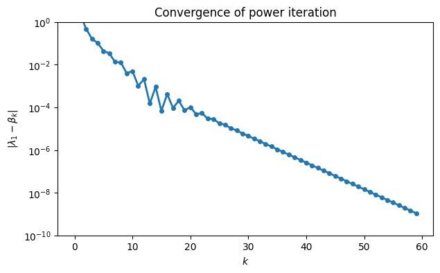

The asymptotic trend seems to be a straight line, consistent with linear convergence. To estimate the convergence rate, we look at the ratio of two consecutive errors in the linear part of the convergence curve. The ratio of the first two eigenvalues should match the observed rate.

print(f"theory: {ev[1] / ev[0]:.5f}")
print(f"observed: {err[40] / err[39]:.5f}")

theory: -0.75000
observed: -0.75511

Note that the error is supposed to change sign on each iteration. The effect of these alternating signs is that estimates oscillate around the exact value.

print(beta[26:30])

[1.0000154  0.99998979 1.00000846 0.99999413]

In practical situations, we don’t know the exact eigenvalue that the algorithm is supposed to find. In that case we would base errors on the final β that was found, as in the following plot.

err = beta[-1] - beta
semilogy(arange(60), abs(err), "-o")
ylim(1e-10, 1), xlabel("$k$")
ylabel("$|\\lambda_1 - \\beta_k|$")
title("Convergence of power iteration");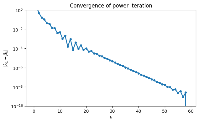

The results are very similar until the last few iterations, when the limited accuracy of the reference value begins to show. That is, while it is a good estimate of $\lambda_1$ , it is less good as an estimate of the error in nearby estimates.

8.3 Inverse iteration¶

Example 8.3.1

We set up a $5\times 5$ triangular matrix with prescribed eigenvalues on its diagonal.

ev = array([1, -0.75, 0.6, -0.4, 0])
A = triu(ones([5, 5]), 1) + diag(ev)    # triangular matrix, eigs on diagonal

We run inverse iteration with the shift $s=0.7$ . Convergence should be to the eigenvalue closest to the shift, which we know to be 0.6 here.

beta, x = FNC.inviter(A, 0.7, 30)
print(beta)

[0.69949953 0.5788059  0.60902175 0.59730106 0.60094685 0.59969144
 0.6001039  0.59996552 0.60001152 0.59999616 0.60000128 0.59999957
 0.60000014 0.59999995 0.60000002 0.59999999 0.6        0.6
 0.6        0.6        0.6        0.6        0.6        0.6
 0.6        0.6        0.6        0.6        0.6        0.6       ]

As expected, the eigenvalue that was found is the one closest to 0.7. The convergence is again linear.

err = beta[-1] - beta    # last estimate is our best
semilogy(arange(30), abs(err), "-o")
ylim(1e-16, 1)
xlabel("$k$"),  ylabel("$|\\lambda_3 - \\beta_k|$")
title(("Convergence of inverse iteration"));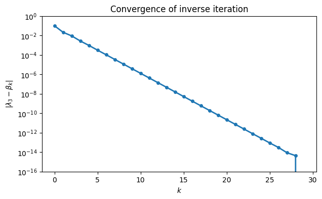

Let’s reorder the eigenvalues to enforce (8.3.3).

ev = ev[argsort(abs(ev - 0.7))]
print(ev)

[ 0.6   1.    0.   -0.4  -0.75]

Now it is easy to compare the theoretical and observed linear convergence rates.

print(f"theory: {(ev[0] - 0.7) / (ev[1] - 0.7):.5f}")
print(f"observed: {err[21] / err[20]:.5f}")

theory: -0.33333
observed: -0.33327

Example 8.3.2

ev = array([1, -0.75, 0.6, -0.4, 0])
A = triu(ones([5, 5]), 1) + diag(ev)    # triangular matrix, eigs on diagonal

We begin with a shift $s=0.7$ , which is closest to the eigenvalue 0.6.

from numpy.linalg import solve
s = 0.7
x = ones(5)
y = solve(A - s * eye(5), x)
beta = x[0] / y[0] + s
print(f"latest estimate: {beta:.8f}")

latest estimate: 0.70348139

Note that the result is not yet any closer to the targeted 0.6. But we proceed (without being too picky about normalization here).

s = beta
x = y / y[0]
y = solve(A - s * eye(5), x)
beta = x[0] / y[0] + s
print(f"latest estimate: {beta:.8f}")

latest estimate: 0.56127614

Still not much apparent progress. However, in just a few more iterations the results are dramatically better.

for k in range(4):
    s = beta
    x = y / y[0]
    y = solve(A - s * eye(5), x)
    beta = x[0] / y[0] + s
    print(f"latest estimate: {beta:.12f}")

latest estimate: 0.596431288475
latest estimate: 0.599971709182
latest estimate: 0.599999997856
latest estimate: 0.600000000000

8.4 Krylov subspaces¶

Example 8.4.1

First we define a triangular matrix with known eigenvalues, and a random vector $b$ .

ev = 10 + arange(1, 101)
A = triu(random.rand(100, 100), 1) + diag(ev)
b = random.rand(100)

Next we build up the first ten Krylov matrices iteratively, using renormalization after each matrix-vector multiplication.

Km = zeros([100, 30])
Km[:, 0] = b
for m in range(29):
    v = A @ Km[:, m]
    Km[:, m + 1] = v / norm(v)

Now we solve least-squares problems for Krylov matrices of increasing dimension, recording the residual in each case.

from numpy.linalg import lstsq
resid = zeros(30)
resid[0] = norm(b)
for m in range(1, 30):
    z = lstsq(A @ Km[:, :m], b, rcond=None)[0]
    x = Km[:, :m] @ z
    resid[m] = norm(b - A @ x)

The linear system approximations show smooth linear convergence at first, but the convergence stagnates after only a few digits have been found.

semilogy(range(30), resid, "-o")
xlabel("$m$"),  ylabel("$\\| b-Ax_m \\|$")
title(("Residual for linear systems"));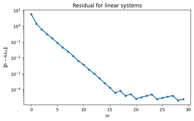

Example 8.4.2

We illustrate a few steps of the Arnoldi iteration for a small matrix.

A = random.choice(range(10), (6, 6))
print(A)

[[1 3 7 3 9 7]
 [0 8 4 9 8 6]
 [8 1 9 9 5 1]
 [5 9 4 3 6 3]
 [8 8 6 7 5 2]
 [3 8 4 6 8 5]]

The seed vector we choose here determines the first member of the orthonormal basis.

u = random.randn(6)
Q = zeros([6, 3])
Q[:, 0] = u / norm(u)

Multiplication by $\mathbf{A}$ gives us a new vector in $\mathcal{K}_2$ .

Aq = A @ Q[:, 0]

We subtract off its projection in the previous direction. The remainder is rescaled to give us the next orthonormal column.

v = Aq - dot(Q[:, 0], Aq) * Q[:, 0]
Q[:, 1] = v / norm(v)

On the next pass, we have to subtract off the projections in two previous directions.

Aq = A @ Q[:, 1]
v = Aq - dot(Q[:, 0], Aq) * Q[:, 0] - dot(Q[:, 1], Aq) * Q[:, 1]
Q[:, 2] = v / norm(v)

At every step, $\mathbf{Q}_m$ is an ONC matrix.

print(f"should be near zero: {norm(Q.T @ Q - eye(3)):.2e}")

should be near zero: 1.37e-15

And $\mathbf{Q}_m$ spans the same space as the three-dimensional Krylov matrix.

from numpy.linalg import matrix_rank
K = stack([u, A @ u, A @ A @ u], axis=-1)
Q_and_K = hstack([Q, K])
print(matrix_rank(Q_and_K))

8.5 GMRES¶

Example 8.5.1

We define a triangular matrix with known eigenvalues and a random vector $\mathbf{b}$ .

ev = 10 + arange(1, 101)
A = triu(random.rand(100, 100), 1) + diag(ev)
b = random.rand(100)

Instead of building the Krylov matrices, we use the Arnoldi iteration to generate equivalent orthonormal vectors.

Q, H = FNC.arnoldi(A, b, 60)
print(H[:5, :5])

[[77.37734323 37.68198103  7.76623215  1.4210155  -1.1732659 ]
 [19.64964842 54.58286026 32.01581406  1.42820014 -0.16509739]
 [ 0.         25.90932193 57.80119766 25.28685492  0.73134252]
 [ 0.          0.         21.98286939 62.9391178  25.25320201]
 [ 0.          0.          0.         23.81918315 55.34041208]]

The Arnoldi bases are used to solve the least-squares problems defining the GMRES iterates.

from numpy.linalg import lstsq
resid = zeros(61)
resid[0] = norm(b)
for m in range(1, 61):
    s = hstack([norm(b), zeros(m)])
    z = lstsq(H[: m + 1, :m], s, rcond=None)[0]
    x = Q[:, :m] @ z
    resid[m] = norm(b - A @ x)

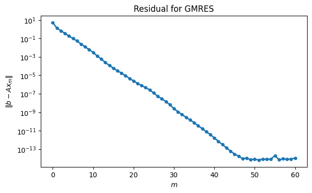
The approximations converge smoothly, practically all the way to machine epsilon.

semilogy(range(61), resid, "-o")
xlabel("$m$"),  ylabel("$\| b-Ax_m \|$")
title("Residual for GMRES");

<>:2: SyntaxWarning: invalid escape sequence '\|'
<>:2: SyntaxWarning: invalid escape sequence '\|'
/var/folders/gc/0752xrm56pnf0r0dsrn5370c0000gr/T/ipykernel_93664/580350478.py:2: SyntaxWarning: invalid escape sequence '\|'
  xlabel("$m$"),  ylabel("$\| b-Ax_m \|$")

Example 8.5.2

The following experiments are based on a matrix resulting from discretization of a partial differential equation.

d = 50;  n = d**2
A = FNC.poisson2d(d)
b = ones(n)
spy(A);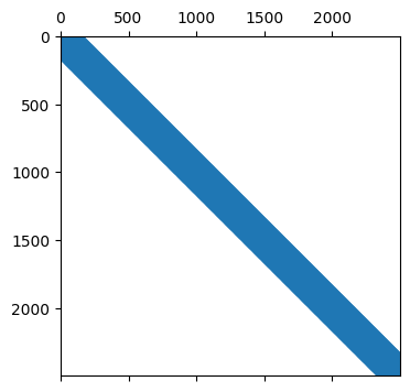

We compare unrestarted GMRES with three different thresholds for restarting. Here we are using gmres from scipy.sparse.linalg, since our simple implementation does not offer restarting. We’re also using a trick to accumulate the vector of residual norms as it runs.

from scipy.sparse.linalg import gmres
ctr = lambda rvec: resid.append(norm(rvec))
resid = [1.]
x, flag = gmres(A, b, restart=None, rtol=1e-8, atol=1e-14, maxiter=120, callback=ctr)
semilogy(resid); 
xlabel("$m$"), ylabel("residual norm")
title(("Convergence of unrestarted GMRES"));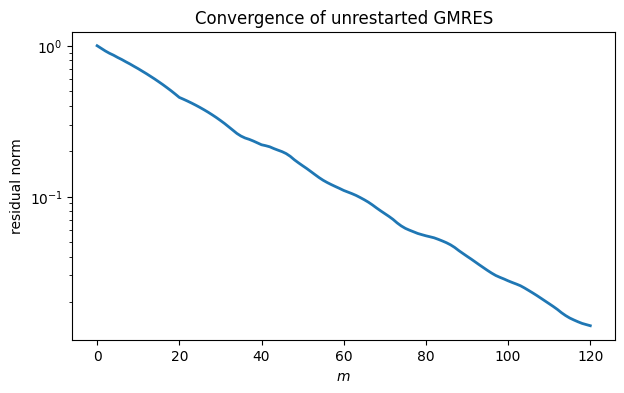

maxit = 120
rtol = 1e-8
restarts = [maxit, 20, 40, 60]
hist = lambda rvec: resid.append(norm(rvec))
for r in restarts:
    resid = [1.]
    x, flag = gmres(A, b, restart=r, rtol=rtol, atol=1e-14, maxiter=maxit, callback=hist)
    semilogy(resid)

ylim(1e-8, 2)
legend(["none", "20", "40", "60"])
title(("Convergence of restarted GMRES"));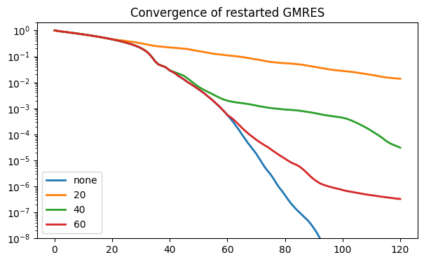

The “pure” GMRES curve is the lowest one. All of the other curves agree with it until the first restart. Decreasing the restart value makes the convergence per iteration generally worse, but the time required per iteration smaller as well.

8.6 MINRES and conjugate gradients¶

Example 8.6.2

The following matrix is indefinite.

from numpy.linalg import eig
import scipy.sparse as sp
A = FNC.poisson2d(10) - 20*sp.eye(100)
ev, _ = eig(A.todense())
num_negative_ev = sum(ev < 0)
print(f"There are {sum(ev < 0)} negative and {sum(ev > 0)} positive eigenvalues")

There are 13 negative and 87 positive eigenvalues

We can compute the relevant quantities from Theorem 8.6.1.

m, M = min(-ev[ev < 0]), max(-ev[ev < 0])
kappa_minus = M / m
m, M = min(ev[ev > 0]), max(ev[ev > 0])
kappa_plus = M / m
S = sqrt(kappa_plus * kappa_minus)
rho = sqrt((S - 1) / (S + 1))
print(f"Condition numbers: {kappa_minus:.2e}, {kappa_plus:.2e}")
print(f"Convergence rate: {rho:.3f}")

Condition numbers: 1.02e+01, 3.76e+01
Convergence rate: 0.950

Because the iteration number $m$ is halved in (8.6.4), the rate constant of linear convergence is the square root of this number, which makes it even closer to 1.

Now we apply MINRES to a linear system with this matrix, and compare the observed convergence to the upper bound from the theorem.

from scipy.sparse.linalg import minres
b = random.rand(100)
resid = [norm(b)]
hist = lambda x: resid.append(norm(b - A @ x))
x, flag = minres(A, b, rtol=1e-8, maxiter=1000, callback=hist)

semilogy(resid, ".-");
upper = norm(b) * rho**arange(len(resid))
semilogy(upper, "k--")
xlabel("$m$"),  ylabel("residual norm")
legend(["MINRES", "upper bound"], loc="lower left")
title("Convergence of MINRES");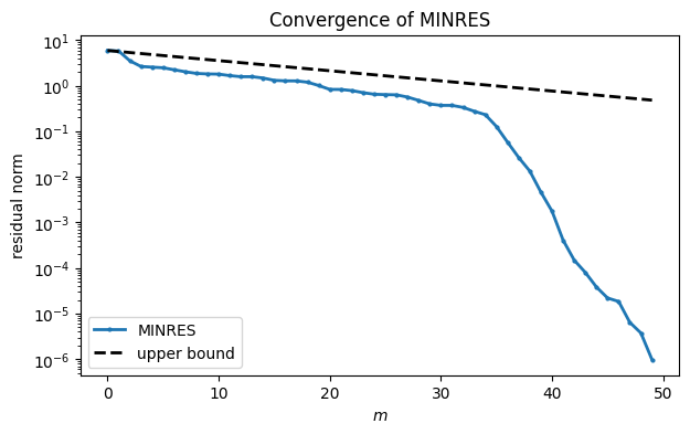

The upper bound turns out to be pessimistic here, especially in the later iterations. However, you can see a slow linear phase in the convergence that tracks the bound closely.

Example 8.6.3

We will compare MINRES and CG on some quasi-random SPD problems. The first matrix has a condition number of 100.

n = 5000
density = 0.001
A = FNC.sprandsym(n, density, rcond=1e-2)
x = arange(1, n+1) / n
b = A @ x

Now we apply both methods and compare the convergence of the system residuals, using implementations imported from scipy.sparse.linalg.

from scipy.sparse.linalg import cg, minres
hist = lambda x: resid.append(norm(b - A @ x))

resid = [norm(b)]
xMR, flag = minres(A, b, rtol=1e-12, maxiter=100, callback=hist)
semilogy(resid / norm(b), label="MINRES")

resid = [norm(b)]
xCG, flag = cg(A, b, rtol=1e-12, maxiter=100, callback=hist)
semilogy(resid / norm(b), label="CG")

xlabel("Krylov dimension $m$"), ylabel("$\\|r_m\\| / \\|b\\|$")
grid(),  legend(),  title("Convergence of MINRES and CG");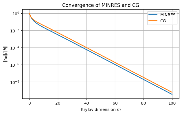

There is little difference between the two methods here. Both achieve relative residual of 10^-6 in aout 60 iterations, for example. The final errors are similar, too.

print(f"MINRES error: {norm(xMR - x) / norm(x):.2e}")
print(f"CG error: {norm(xCG - x) / norm(x):.2e}")

MINRES error: 4.68e-09
CG error: 2.98e-09

Next, we increase the condition number of the matrix by a factor of 25. The rule of thumb predicts that the number of iterations required should increase by a factor of about 5; i.e., 300 iterations to reach 10^-6.

A = FNC.sprandsym(n, density, rcond=1e-2 / 25)
x = arange(1, n+1) / n
b = A @ x

from scipy.sparse.linalg import cg, minres
hist = lambda x: resid.append(norm(b - A @ x))

resid = [norm(b)]
xMR, flag = minres(A, b, rtol=1e-12, maxiter=400, callback=hist)
semilogy(resid / norm(b), label="MINRES")

resid = [norm(b)]
xCG, flag = cg(A, b, rtol=1e-12, maxiter=400, callback=hist)
semilogy(resid / norm(b), label="CG")

xlabel("Krylov dimension $m$"), ylabel("$\\|r_m\\| / \\|b\\|$")
grid(),  legend(),  title("Convergence of MINRES and CG")

print(f"MINRES error: {norm(xMR - x) / norm(x):.2e}")
print(f"CG error: {norm(xCG - x) / norm(x):.2e}")

MINRES error: 2.52e-07
CG error: 1.50e-07

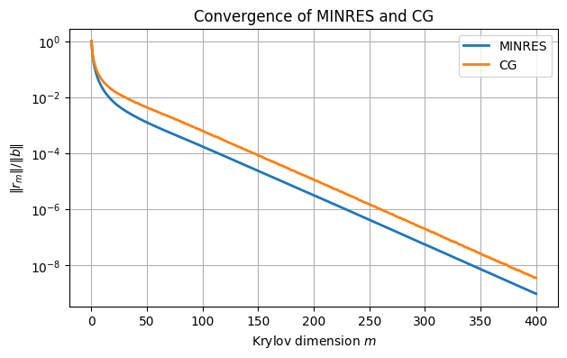
Both methods have an early superlinear phase that allow them to finish slightly sooner than the factor of 5 predicted: Theorem 8.6.2 is an upper bound, not necessarily an approximation.

8.7 Matrix-free iterations¶

Example 8.7.1

We use a readily available test image.

from skimage import data as testimages
from skimage.color import rgb2gray
img = getattr(testimages, "coffee")()
X = rgb2gray(img)
imshow(X, cmap="gray");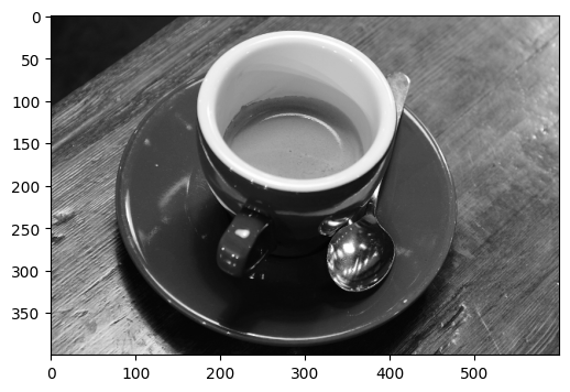

We define the one-dimensional tridiagonal blurring matrices.

import scipy.sparse as sp
def blurmatrix(d):
    data = [[0.25] * (d-1), [0.5] * d, [0.25] * (d-1)]
    return sp.diags(data, [-1, 0, 1], shape=(d, d))

m, n = X.shape
B = blurmatrix(m)
C = blurmatrix(n)

Finally, we show the results of using $k=12$ repetitions of the blur in each direction.

from scipy.sparse.linalg import matrix_power
blur = lambda X: matrix_power(B, 12) @ X @ matrix_power(C, 12)

imshow(blur(X), cmap="gray")
title("Blurred image");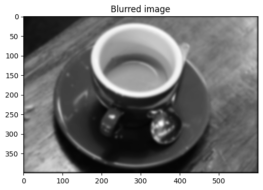

Example 8.7.2

We repeat the earlier process to blur an original image $\mathbf{X}$ to get $\mathbf{Z}$ .

img = getattr(testimages, "coffee")()
X = rgb2gray(img)
m, n = X.shape

import scipy.sparse as sp
def blurmatrix(d):
    data = [[0.25] * (d-1), [0.5] * d, [0.25] * (d-1)]
    return sp.diags(data, [-1, 0, 1], shape=(d, d))
B = blurmatrix(m)
C = blurmatrix(n)

from scipy.sparse.linalg import matrix_power
blur = lambda X: matrix_power(B, 12) @ X @ matrix_power(C, 12)

Z = blur(X)
imshow(Z, cmap="gray")
title("Blurred image");

Now we imagine that $\mathbf{X}$ is unknown and that we want to recover it from $\mathbf{Z}$ . We first need functions that translate between vector and matrix representations.

from scipy.sparse.linalg import LinearOperator
vec = lambda Z: Z.reshape(m * n)
unvec = lambda z: z.reshape(m, n)
xform = lambda x: vec(blur(unvec(x)))

Now we declare the three-step blur transformation as a LinearOperator, supplying also the size of the vector form of an image.

T = LinearOperator((m * n, m * n), matvec=xform)

The blurring operators are symmetric, so we apply minres to the composite blurring transformation T.

from scipy.sparse.linalg import gmres
y, flag = gmres(T, vec(Z), rtol=1e-5, maxiter=50)
Y = unvec(maximum(0, minimum(1, y)))


subplot(1, 2, 1),  imshow(X, cmap="gray")
axis("off"),  title("Original")
subplot(1, 2, 2),  imshow(Y, cmap="gray")
axis("off"),  title("Deblurred");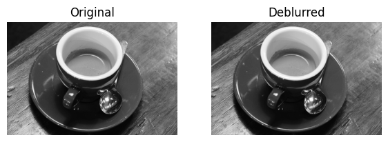

8.8 Preconditioning¶

Example 8.8.1

Here is an SPD matrix that arises from solving partial differential equations.

from scipy.sparse import sparray
import rogues
A = rogues.wathen(60, 60)
n = A.shape[0]
print(f"Matrix is {n} x {n} with {A.nnz} nonzeros")

Matrix is 11041 x 11041 with 170161 nonzeros

There is an easy way to use the diagonal elements of $\mathbf{A}$ , or any other vector, as a diagonal preconditioner.

import scipy.sparse as sp
prec = sp.diags(1 / A.diagonal(), 0)

We now compare CG with and without the preconditioner.

from scipy.sparse.linalg import cg
b = ones(n)
hist = lambda x: resid.append(norm(b - A @ x))
resid = [norm(b)]
start = timer()
x, _ = cg(A, b, rtol=1e-4, maxiter=200, callback=hist)
print(f"No preconditioner: Finished in {timer() - start:.2f} sec")
resid_plain = resid.copy()
resid = [norm(b)]
start = timer()
x, _ = cg(A, b, rtol=1e-4, maxiter=200, M=prec, callback=hist)
print(f"Diagonal preconditioner: Finished in {timer() - start:.2f} sec")
resid_prec = resid.copy()

semilogy(resid_plain, label="no preconditioner")
semilogy(resid_prec, label="diagonal preconditioner")
xlabel("iteration"), ylabel("residual norm")
legend(),  title("Convergence of CG with and without preconditioning");

No preconditioner: Finished in 2.94 sec

Diagonal preconditioner: Finished in 0.59 sec

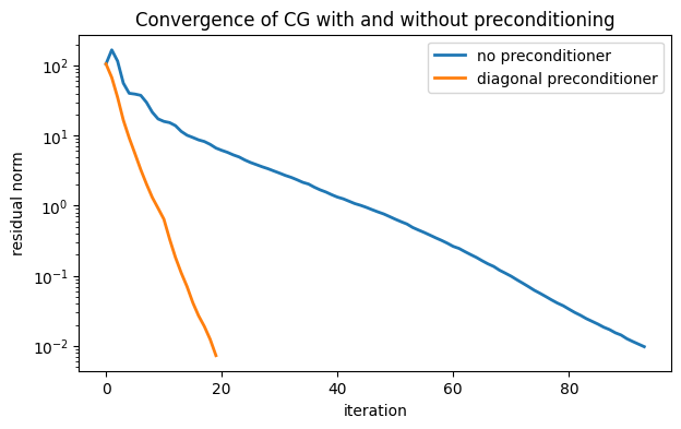
The diagonal preconditioner cut down substantially on the number of iterations and the execution time.

Example 8.8.2

Here is a random nonsymmetric matrix.

import scipy.sparse as sp
n = 8000
A = 2.8 * sp.eye(n) + sp.rand(n, n, 0.002)

Without a preconditioner, GMRES can solve a system with this matrix.

from scipy.sparse.linalg import gmres

b = random.rand(n)
hist = lambda rvec: resid.append(norm(rvec))
resid = [1.]

start = timer()
x, flag = gmres(A, b, maxiter=300, rtol=1e-10, restart=50, callback=hist)
print(f"time for plain GMRES: {timer() - start:.3f} sec")
resid_plain = resid.copy()

time for plain GMRES: 0.209 sec

The following version of incomplete LU factorization drops all sufficiently small values (i.e., replaces them with zeros). This keeps the number of nonzeros in the factors under control.

from scipy.sparse.linalg import spilu
iLU = spilu(A, drop_tol=0.2)
print(f"Factors have {iLU.nnz} nonzeros, while A has {A.nnz}")

/var/folders/gc/0752xrm56pnf0r0dsrn5370c0000gr/T/ipykernel_93664/769705972.py:2: SparseEfficiencyWarning: spilu converted its input to CSC format
  iLU = spilu(A, drop_tol=0.2)

Factors have 100036 nonzeros, while A has 135987

The result is not a true factorization of the original matrix. However, it’s close enough for an approximate inverse in a preconditioner.

from scipy.sparse.linalg import LinearOperator
prec = LinearOperator((n, n), matvec=lambda y: iLU.solve(y))

resid = [1.];  start = timer()
x, flag = gmres(A, b, M=prec, maxiter=300, rtol=1e-10, restart=50, callback=hist)
print(f"time for preconditioned GMRES: {timer() - start:.3f} sec")
resid_prec = resid

time for preconditioned GMRES: 0.142 sec

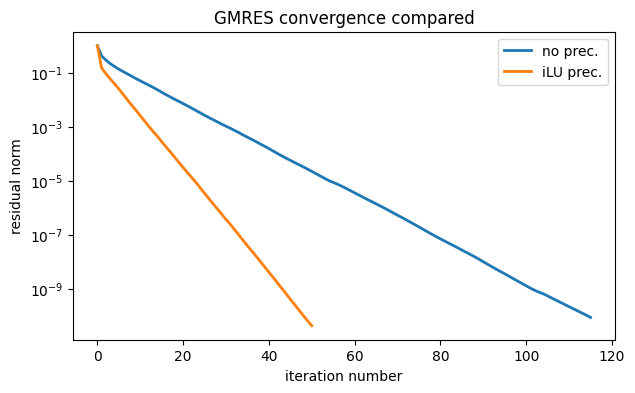
semilogy(resid_plain, label="no prec.")
semilogy(resid_prec, label="iLU prec.")
xlabel("iteration number"),  ylabel("residual norm")
legend()
title("GMRES convergence compared");