Examples
7.1 From matrix to insight
Example 7.1.4
Here we create an adjacency matrix for a graph on four nodes.
A = array([[0, 1, 0, 0], [1, 0, 0, 0], [1, 1, 0, 1], [0, 1, 1, 0]])
print(A)
[[0 1 0 0]
[1 0 0 0]
[1 1 0 1]
[0 1 1 0]]
The networkx package has many functions for working with graphs. Here, we instruct it to create a directed graph from the adjacency matrix, then make a drawing of it.
import networkx as nx
G = nx.from_numpy_array(A, create_using=nx.DiGraph)
nx.draw(G, with_labels=True, node_color="yellow")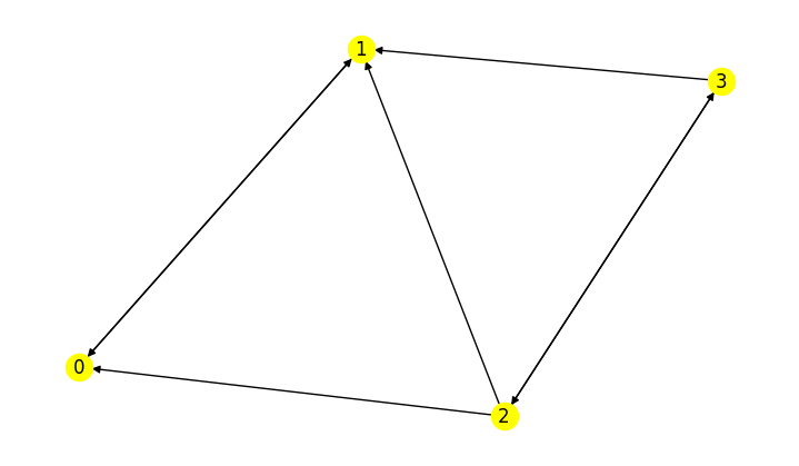
Here are the counts of all walks of length 3 in the graph:
print(A**3)[[0 1 0 0]
[1 0 0 0]
[1 1 0 1]
[0 1 1 0]]
If the adjacency matrix is symmetric, the result is an undirected graph: all edges connect in both directions.
A = array([[0, 1, 1, 0], [1, 0, 0, 1], [1, 0, 0, 0], [0, 1, 0, 0]])
G = nx.from_numpy_array(A, create_using=nx.Graph)
nx.draw(G, with_labels=True, node_color="yellow")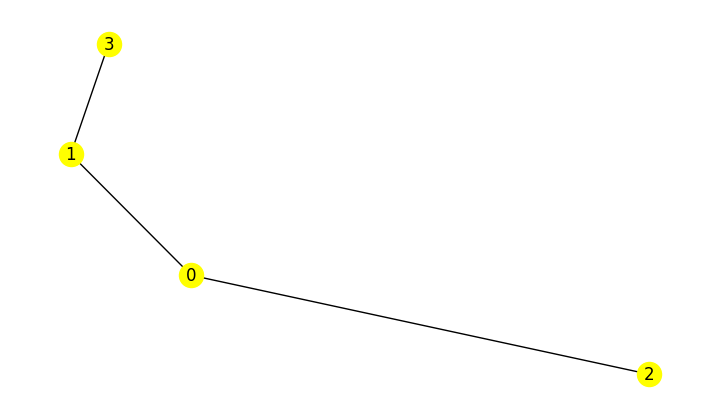
Example 7.1.5
We will use a test image from the well-known scikit-image package.
from skimage import data as testimages
img = getattr(testimages, "coffee")()
imshow(img)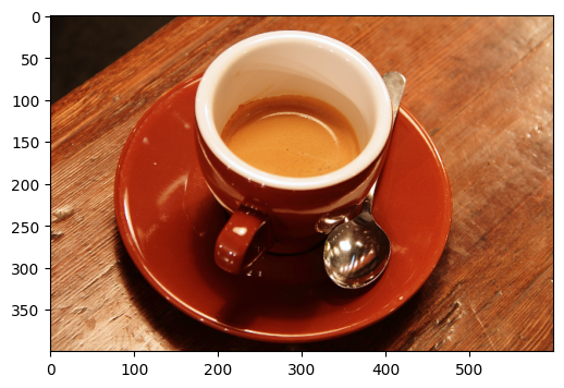
The variable img is a matrix.
size(img)720000However, its entries are colors, not numbers.
print(f"image has shape {img.shape}")
print(f"first pixel has value {img[0, 0]}")
image has shape (400, 600, 3)
first pixel has value [21 13 8]
The three values at each pixel are for intensities of red, green, and blue. We can convert each of those layers into an ordinary matrix of values between 0 and 255, which is maximum intensity.
R = img[:, :, 0]
print("upper left corner of the red plane is:")
print(R[:5, :5])
print(f"red channel values range from {R.min()} to {R.max()}")
upper left corner of the red plane is:
[[21 21 20 21 21]
[21 21 20 22 20]
[21 23 20 21 21]
[21 21 21 21 20]
[21 21 21 21 21]]
red channel values range from 0 to 255
It may also be convenient to convert the image to grayscale, which has just one layer of values from zero (black) to one (white).
from skimage.color import rgb2gray
A = rgb2gray(img)
A[:5, :5]
print("upper left corner of grayscale:")
print(A[:5, :5])
print(f"gray values range from {A.min()} to {A.max()}")
upper left corner of grayscale:
[[0.05623333 0.05651608 0.04978902 0.05708157 0.05903882]
[0.05595059 0.05651608 0.05792275 0.05987216 0.05511725]
[0.05875608 0.05846549 0.05848824 0.05651608 0.06212706]
[0.05566784 0.05651608 0.05623333 0.05679882 0.05174627]
[0.0553851 0.05595059 0.05510235 0.05595059 0.05623333]]
gray values range from 0.0002827450980392157 to 1.0
imshow(A, cmap='gray')
axis('off');
Some changes we make to the grayscale matrix are easy to interpret visually.
imshow(flipud(A), cmap='gray')
axis('off');
7.2 Eigenvalue decomposition
Example 7.2.2
The eig function from scipy.linalg will return a vector of eigenvalues and a matrix of associated eigenvectors.
from numpy.linalg import eig
A = pi * ones([2, 2])
d, V = eig(A)
print("eigenvalues:", d)
eigenvalues: [ 6.28318531e+00 -6.97573700e-16]
We can check the fact that this is an EVD (although in practice we never invert a matrix).
from numpy.linalg import inv
D = diag(d)
print(f"should be near zero: {norm(A - V @ D @ inv(V), 2):.2e}")
should be near zero: 1.26e-15
If the matrix is not diagonalizable, no message is given, but V will be singular. The robust way to detect that circumstance is via .
from numpy.linalg import cond
A = array([[1, 1], [0, 1]])
d, V = eig(A)
print(f"cond(V) is {cond(V):.2e}")
cond(V) is 9.01e+15
But even in the nondiagonalizable case, holds up to roundoff error.
print(f"should be near zero: {norm(A @ V - V @ diag(d), 2):.2e}")should be near zero: 2.22e-16
Example 7.2.3
We first define a hermitian matrix. Note that we add the conjugate transpose of a matrix to itself.
n = 7
A = random.randn(n, n) + 1j * random.randn(n, n)
A = (A + conj(A.T)) / 2
We confirm that the matrix is normal by checking that (to within roundoff).
from numpy.linalg import eig
d, V = eig(A)
print(f"eigenvector matrix has condition number {cond(V):.5f}")
eigenvector matrix has condition number 1.00000
Now we perturb and measure the effect on the eigenvalues. Note that the Bauer–Fike theorem uses absolute differences, not relative ones. Since the ordering of eigenvalues can change, we look at all pairwise differences and take the minima.
E = random.randn(n, n) + 1j * random.randn(n, n)
E = 1e-8 * E / norm(E, 2)
dd, _ = eig(A + E)
dist = array([min([abs(x - y) for x in dd]) for y in d])
print(dist)
[9.13062970e-10 3.34658175e-09 7.06122371e-10 4.31937276e-10
1.05432865e-09 3.97864390e-09 2.06839348e-09]
As promised, the perturbations in the eigenvalues do not exceed the normwise perturbation to the original matrix.
Now we see what happens for a triangular matrix.
n = 20
x = arange(n) + 1
A = triu(outer(x, ones(n)))
print(A[:5, :5])
[[1. 1. 1. 1. 1.]
[0. 2. 2. 2. 2.]
[0. 0. 3. 3. 3.]
[0. 0. 0. 4. 4.]
[0. 0. 0. 0. 5.]]
This matrix is not at all close to normal.
d, V = eig(A)
print(f"eigenvector matrix has condition number {cond(V):.2e}")
eigenvector matrix has condition number 6.15e+09
As a result, the eigenvalues can change by a good deal more.
E = random.randn(n, n) + 1j * random.randn(n, n)
E = 1e-8 * E / norm(E, 2)
dd, _ = eig(A + E)
dist = array([min([abs(x - y) for x in dd]) for y in d])
print(f"Maximum eigenvalue change is {max(dist):.2e}")
print(f"The Bauer-Fike upper bound is {cond(V) * norm(E, 2):.2e}")
Maximum eigenvalue change is 8.18e-01
The Bauer-Fike upper bound is 6.15e+01
If we plot the eigenvalues of many perturbations, we get a cloud of points that roughly represents all the possible eigenvalues when representing this matrix with single-precision accuracy.
clf
scatter(d, zeros(n), 18)
axis("equal")
for _ in range(100):
    E = random.randn(n, n) + 1j * random.randn(n, n)
    E = finfo(np.float32).eps * E / norm(E, 2)
    dd, _ = eig(A + E)
    scatter(real(dd), imag(dd), 2, 'k')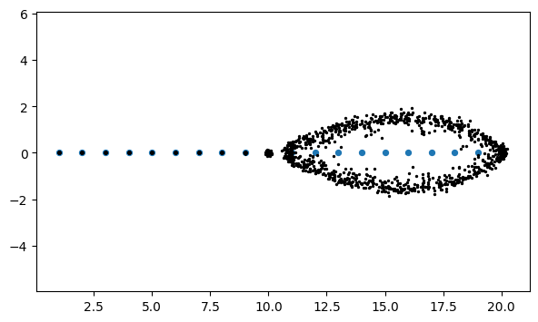
The plot shows that some eigenvalues are much more affected than others. This situation is not unusual, but it is not explained by the Bauer–Fike theorem.
Example 7.2.4
Let’s start with a known set of eigenvalues and an orthogonal eigenvector basis.
from numpy.linalg import qr
D = diag([-6, -1, 2, 4, 5])
V, R = qr(random.randn(5, 5))
A = V @ D @ V.T # note that V.T = inv(V) hereprint(sort(eig(A)[0]))[-6. -1. 2. 4. 5.]
Now we will take the QR factorization and just reverse the factors.
Q, R = qr(A)
A = R @ Q;
It turns out that this is a similarity transformation, so the eigenvalues are unchanged.
print(sort(eig(A)[0]))[-6. -1. 2. 4. 5.]
What’s remarkable, and not elementary, is that if we repeat this transformation many times, the resulting matrix converges to .
for k in range(40):
    Q, R = qr(A)
    A = R @ Q
set_printoptions(precision=4)
print(A)
[[-6.0000e+00 -6.3163e-05 -7.7494e-07 8.0433e-16 -6.6814e-16]
[-6.3163e-05 5.0000e+00 3.4480e-03 1.3223e-15 -1.2786e-16]
[-7.7494e-07 3.4480e-03 4.0000e+00 -2.8128e-13 2.4507e-16]
[ 7.1896e-20 6.4328e-16 -2.8163e-13 2.0000e+00 3.8647e-13]
[-3.5579e-32 -9.6403e-29 1.2418e-26 3.8653e-13 -1.0000e+00]]
7.3 Singular value decomposition
Example 7.3.4
We verify some of the fundamental SVD properties using standard Julia functions from LinearAlgebra.
A = array([[(i + 1.0) ** j for j in range(4)] for i in range(5)])
set_printoptions(precision=4)
print(A)
[[ 1. 1. 1. 1.]
[ 1. 2. 4. 8.]
[ 1. 3. 9. 27.]
[ 1. 4. 16. 64.]
[ 1. 5. 25. 125.]]
The factorization is obtained using svd from numpy.linalg.
from numpy.linalg import svd
U, sigma, Vh = svd(A)
print("singular values:")
print(sigma)
singular values:
[1.4670e+02 5.7386e+00 9.9985e-01 1.1928e-01]
By default, the full factorization type is returned. This can be a memory hog if one of the dimensions of is very large.
print("size of U:", U.shape)
print("size of V:", Vh.T.shape)
size of U: (5, 5)
size of V: (4, 4)
Both and are orthogonal (in the complex case, unitary). Note that it’s that is returned, not .
print(f"should be near zero: {norm(U.T @ U - eye(5), 2):.2e}")
print(f"should be near zero: {norm(Vh @ Vh.T - eye(4), 2):.2e}")
should be near zero: 5.61e-16
should be near zero: 1.07e-15
Next we test that we have the factorization promised by the SVD, using diagsvd to construct a rectangular diagonal matrix.
from scipy.linalg import diagsvd
S = diagsvd(sigma, 5, 4)
print(f"should be near zero: {norm(A - U @ S @ Vh, 2):.2e}")
should be near zero: 8.56e-14
Here is verification of the connections between the singular values, norm, and condition number.
from numpy.linalg import cond
print("largest singular value:", sigma[0])
print("2-norm of the matrix:  ", norm(A, 2))
print("singular value ratio:", sigma[0] / sigma[-1])
print("2-norm condition no.:", cond(A, 2))
largest singular value: 146.69715365883005
2-norm of the matrix: 146.69715365883005
singular value ratio: 1229.8468876337527
2-norm condition no.: 1229.8468876337529
For matrices that are much taller than they are wide, the thin SVD form is more memory-efficient, because takes the same shape.
A = random.randn(1000, 10)
U, sigma, Vh = svd(A, full_matrices=False)
print("size of U:", U.shape)
print("size of V:", Vh.shape)
size of U: (1000, 10)
size of V: (10, 10)
7.4 Symmetry and definiteness
Example 7.4.1
We will use a symmetric matrix with a known EVD and eigenvalues equal to the integers from 1 to 20.
from numpy.linalg import qr
n = 20
d = arange(n) + 1
D = diag(d)
V, _ = qr(random.randn(n, n))    # get a random orthogonal V
A = V @ D @ V.T
The Rayleigh quotient is a scalar-valued function of a vector.
R = lambda x: dot(x, A @ x) / dot(x, x)The Rayleigh quotient evaluated at an eigenvector gives the corresponding eigenvalue.
print(R(V[:, 6]))7.0
If the input to he Rayleigh quotient is within a small δ of an eigenvector, its output is within of the corresponding eigenvalue. In this experiment, we observe that each additional digit of accuracy in an approximate eigenvector gives two more digits to the eigenvalue estimate coming from the Rayleigh quotient.
results = PrettyTable(["perturbation size", "R.Q. - λ"])
for delta in 1 / 10 ** arange(1, 6):
    e = random.randn(n)
    e = delta * e / norm(e)
    x = V[:, 5] + e
    quotient = R(x)
    results.add_row([delta, quotient - d[5]])

print(results)
+-------------------+------------------------+
| perturbation size | R.Q. - λ |
+-------------------+------------------------+
| 0.1 | 0.035247810976065885 |
| 0.01 | 0.0003015262874548341 |
| 0.001 | 5.558704769370593e-06 |
| 0.0001 | 4.121216701236108e-08 |
| 1e-05 | 3.9184655520330125e-10 |
+-------------------+------------------------+
7.5 Dimension reduction
Example 7.5.1
We make an image from some text, then reload it as a matrix.
text(
    0.5,
    0.5,
    "Hello world",
    dict(fontsize=44),
    horizontalalignment="center",
    verticalalignment="center",
)
axis("off")
savefig("hello.png")
img = imread("hello.png")[:, :, :3]
A = rgb2gray(img)
print(f"image of size {A.shape}")
image of size (400, 700)
Next we show that the singular values decrease until they reach zero (more precisely, until they are about times the norm of the matrix) at around index 38.
from numpy.linalg import svd
U, sigma, Vt = svd(A)
semilogy(sigma, "o")
title("Singular values")
xlabel("$i$"), ylabel("$\\sigma_i$");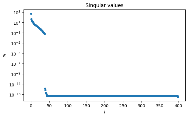
significant = sigma / sigma[0] > 10 * 2**-52
print(f"last significant singular value at index {max(where(significant)[0])}")
last significant singular value at index 38
The rapid decrease suggests that we can get fairly good low-rank approximations.
for k in range(4):
    r = 2 + 2 * k
    Ak = U[:, :r] @ diag(sigma[:r]) @ Vt[:r, :]
    subplot(2, 2, k + 1)
    imshow(Ak, cmap="gray", clim=(0.0, 1.0))
    title(f"rank = {r}")
    xticks([]), yticks([])
Consider how little data is needed to reconstruct these images. For rank-8, for instance, we have 8 left and right singular vectors plus 8 singular values.
m, n = A.shape
full_size = m * n
compressed_size = 8 * (m + n + 1)
print(f"compression ratio: {full_size / compressed_size:.1f}")
compression ratio: 31.8
Example 7.5.2
This matrix describes the votes on bills in the 111th session of the United States Senate. (The data set was obtained from [https://
from scipy.io import loadmat
vars = loadmat("voting.mat")
A = vars["A"]
m, n = A.shape
print("size:", (m, n))
size: (112, 696)
If we visualize the votes (yellow is “yea,” blue is “nay”), we can see great similarity between many rows, reflecting party unity.
imshow(A, cmap="viridis")
xlabel("bill")
ylabel("senator")
title("Votes in 111th U.S. Senate");
We use (7.5.4) to quantify the decay rate of the values.
U, sigma, Vt = svd(A)
tau = cumsum(sigma**2) / sum(sigma**2)
plot(range(1, 17), tau[:16], "o")
xlabel("$k$")
ylabel("$\tau_k$")
title("Fraction of singular value energy");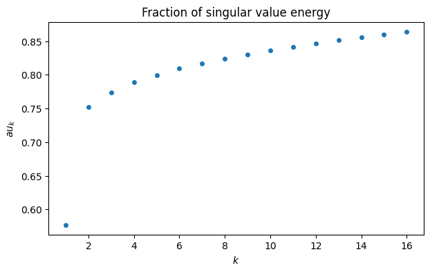
The first and second singular triples contain about 58% and 17%, respectively, of the energy of the matrix. All others have far less effect, suggesting that the information is primarily two-dimensional. The first left and right singular vectors also contain interesting structure.
subplot(1, 2, 1)
plot(U[:, 0], "o")
xlabel("senator"),title("left singular vector")
subplot(1, 2, 2)
plot(Vt[0, :], "o")
xlabel("bill"), title("right singular vector");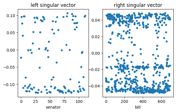
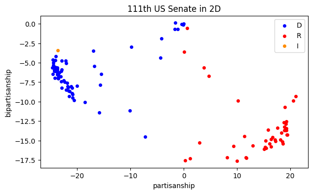
Both vectors have values greatly clustered near for a constant . These can be roughly interpreted as how partisan a particular senator or bill was, and for which political party. Projecting the senators’ vectors into the first two -coordinates gives a particularly nice way to reduce them to two dimensions. Political scientists label these dimensions partisanship and bipartisanship. Here we color them by actual party affiliation (also given in the data file): red for Republican, blue for Democrat, and yellow for independent.
x1 = sigma[0] * U[:, 0]
x2 = sigma[1] * U[:, 1]

Rep = vars["Rep"] - 1
Dem = vars["Dem"] - 1
Ind = vars["Ind"] - 1

scatter(x1[Dem], x2[Dem], color="blue", label="D")
scatter(x1[Rep], x2[Rep], color="red", label="R")
scatter(x1[Ind], x2[Ind], color="darkorange", label="I")

xlabel("partisanship"),  ylabel("bipartisanship")
legend(),  title("111th US Senate in 2D");